Attia Rani | Qazi M. Hssan | Kamran Ayub | Jamshad Ahmad* | Aniqa Zulfiqar
© 2020 IIETA. This article is published by IIETA and is licensed under the CC BY 4.0 license (http://creativecommons.org/licenses/by/4.0/).
OPEN ACCESS
In soliton theory, nonlinear mathematical models and their solutions have great importance due to their geometrical behavior. The major focus of this article is to discover solutions of the traveling wave for the equation of foam drainage and NLEEs of 4th order. The (G'/G)-expansion approach is used on these nonlinear differential equations. With the proper utilization of complex transform these nonlinear PDEs are converted into an ODE. It is noticed that (G'/G)-expansion technique is a sophisticated and accessible tool in engineering, optics, and mathematical physics to find solutions for NLEEs. The method proposed is very efficient and responsible.
method of (G'/G)-expansion, nonlinear evolution equation, solutions of travelling wave, maple 18
We have observed extraordinary progress in the theory of soliton over the past few years. In mathematical physics, a soliton is a self-strengthening solitary wave packet that preserves its shape when it propagates at a continuous speed. Solitons were studied for their application in physical phenomena by mathematicians, physicists and engineers. Soliton waves were first observed by an engineer John Scott Russell. In nature, a number of scientific and physical problems are demonstrated by differential equations which are of great significance. Exact traveling wave solutions of differential equations are one of the important tools for understanding of these nonlinear phenomena as well as applications. To find out the different techniques for solitary wave solutions of partial differential equations is the great success of mathematicians. Exact solutions essentially contribute in nonlinear physical sciences, resultantly, we are able to study physical conduct and discuss further characteristics of the problem that provide track to further applications.
A good approach given by Wang et al that is known as (G'/G)-expansion method, provides the exact traveling wave solutions of nonlinear evolution equations (NLEEs). In this method, a linear ordinary differential equation of 2nd order G'' (η) +σG' (η) +φG (η)=0 is used as the auxiliary equation. (G´/G)-expansion method [1-8] is used for solving numerous types of the nonlinear evolution equations. Duranda and Langevin [9] investigated theoretically the effect of surface viscoelasticity on the drainage of an aqueous foam and presented numericall some solitry wave solutions of drainge equation for intermediate values of new control parameter. A new modification was proposed by Naher et al. [10] in (G´/G)-expansion method to study the higher dimensional modified KdV-Zakharov-Kuznetsev equation. Later, the new extended (G´/G)-expansion method purposed by Roshid has been applied on the (3 + 1)-dimensional potential-YTSF equation [11]. Method of Multiple (G'/G)-expansion was used by Chen and Li [12] in the current year for NLEEs. Wang et al. [13] applied multiple (G'/G)-expansion method to discover Broer-Kaup's traveling wave solutions and approximate long water wave equations. Aslan and Oz ̈is [14] used (G'/G)-expansion method to find out the traveling wave solutions of NLEEs. The solutions are expressed in the proposed method in terms of rational trigonometric, hyperbolic and rational functions. The suggested approach is an important instrument and much user-friendly for obtaining exact solutions of NLEEs. For exact solutions, Yang [15] proposed a new integral transform to find the analytical solution of heat diffusion problem and also Yang [16] introduced a technology as new integral transform method to find the solution for the differential equation in the steady heat transfer Problem. Furthermore, Yang et al. [17] presented an original study on exact travelling wave solutions of non-differentiable type of local fractional Korteweg-de Vries equation and Yang et al. [18] examined the exact travelling wave solutions via e local fractional Riccati differential equation method using travelling wave transformation of the non-differentiable type problems.
The nonlinear PDE in the general form can be expressed as
$\bar{O}\left(\begin{array}{c}\bar{h}, \bar{h}_{t}, \bar{h}_{x}, \bar{h}_{y}, \bar{h}_{z}, \bar{h}_{t t}, \bar{h}_{x x}, \bar{h}_{y y}, \bar{h}_{x x}, \bar{h}_{x t} \\ \bar{h}_{y t}, \bar{h}_{z t}, \bar{h}_{x y}, \bar{h}_{x z}, \bar{h}_{y z}, \ldots\end{array}\right)=0$. (1)
Here $\bar{O}$ is polynomial in $\bar{m}(x, t)$. The method of (G´/G)-expansion is as follows:
Step 1: Reduce Eq. (1) into ordinary differential equation by assuming the wave transformation
$\bar{h}(x, t)=\bar{h}(\bar{\xi}), \bar{\xi}=k x+l y+m z+\omega t$. (2)
and Eq. (1) change into the ODE.
$Q\left(\bar{h}, \bar{h}^{\prime}, \bar{h}^{\prime \prime}, \bar{h}^{\prime \prime \prime}, \ldots\right)=0$. (3)
where, superscripts represent the derivative of $\bar{h}$ w.r.t. $\bar{\xi}$ and ω represents constant.
Step 2: It is possible to obtain constant of integration (s) by integrating Eq. (3) sequentially, if feasible, one or more times. The constant of integration (s) may be fixed to 0 for minimalism.
Step 3: Suppose that the wave solution can be written as follows, according to the proposed algorithm.
$\bar{h}(\xi)=a_{0}+\sum_{n=1}^{M} a_{n}\left(\frac{G^{\prime}}{G}\right)^{n}$. (4)
where, G is the solution of first order nonlinear equation in the following form:
$G^{\prime \prime}+\sigma G^{\prime}+\varphi G=0$. (5)
Unknown constants are σ and φ. General solution is used in Eq. (4), we get
$\frac{G^{\prime}(\bar{\xi})}{G(\bar{\xi})}=\left\{\begin{array}{c}\frac{\sqrt{\sigma^{2}-4 \varphi}}{2}\left(\frac{c_{1} \sinh \left(\frac{1}{2} \sqrt{\sigma^{2}-4 \varphi \bar{\xi}}\right)+c_{2} \cosh \left(\frac{1}{2} \sqrt{\sigma^{2}-4 \varphi \bar{\xi}}\right)}{c_{1} \cosh \left(\frac{1}{2} \sqrt{\sigma^{2}-4 \varphi}\right)+c_{2} \sinh \left(\frac{1}{2} \sqrt{\sigma^{2}-4 \varphi \bar{\xi}}\right)}\right)-\frac{\sigma}{2}, \\ \frac{\sqrt{-\sigma^{2}+4 \varphi}}{2}\left(\frac{-c_{1} \sin \left(\frac{1}{2} \sqrt{-\sigma^{2}+4 \varphi \bar{\xi}}\right)+c_{2} \cos \left(\frac{1}{2} \sqrt{-\sigma^{2}+4 \varphi \bar{\xi}}\right)}{c_{1} \cos \left(\frac{1}{2} \sqrt{-\sigma^{2}+4 \varphi \bar{\xi}}\right)+c_{2} \sin \left(\frac{1}{2} \sqrt{-\sigma^{2}+4 \varphi \bar{\xi}}\right)}\right)-\frac{\sigma}{2}, \\ \sigma^{2}-4 \varphi<0. \\ \frac{2 c_{1}}{c_{1}+c_{2} \bar{\xi}}-\frac{\sigma}{2}, \sigma^{2}-4 \varphi=0.\end{array}\right.$ (6)
where, c1, c2 are unknown constants and, we have
$\left(\frac{G^{\prime}(\bar{\xi})}{G(\bar{\xi})}\right)^{\prime}=-\left[\left(\frac{G^{\prime}}{G}\right)^{2}+\sigma\left(\frac{G^{\prime}}{G}\right)+\varphi\right]$.
$\left(\frac{G^{\prime}(\bar{\xi})}{G(\bar{\xi})}\right)^{\prime \prime}=\left[2\left(\frac{G^{\prime}}{G}\right)^{3}+3 \sigma\left(\frac{G^{\prime}}{G}\right)^{2}+\left(\sigma^{2}+2 \varphi\right)\left(\frac{G^{\prime}}{G}\right)+\varphi \lambda\right]$,
where, the derivatives w.r.t $\bar{\xi}$ have defined the primes. We follow these four steps to find out $\bar{h}$ explicitly.
Step 4: Using Eq. (4) and (5) into Eq. (3) get all values together with the identical order of (G'/G), the left-hand side of the Eq. (1) is changed into a polynomial in (G'/G). After this by putting each coefficient of this polynomial equal to 0 gives a system of algebraic equations by using MAPLE 18 for k, l, m, w, ԑ and an, n=0.1, …, M.
Step 5: Then solve the obtained set of the algebraic equations for k, l, m, ω, ԑ and an, n=0.1, …, M with the help of Maple 18.
Step 6: Use these obtained results from the preceding steps to get a series of fundamental solutions $\bar{h}(\bar{\xi})$ of equation (3) which is depending on (G′/G). Since the solutions of Eq. (4) will be known for us, and then we can be able to attain the exact solutions of Eq. (5).
To demonstrate the method of (G′/G) expansion method we solve the following two problems.
3.1 Equation of foam drainage
Assume the equation of Foam drainage [9]
$\frac{\partial \eta}{\partial t}+\frac{\partial}{\partial x}\left(\eta^{2}-\frac{\sqrt{\eta}}{2} \frac{\partial \eta}{\partial x}\right)=0$. (7)
Here time coordinates (t) and scaled position (x) express the channel formed of a cross-section at the intersection spot from three films, mostly referred to as the border of the plateau (Channels filled with liquid). We concentrate on measurable detail of coupling of drainage. Foam effluent is the movement of fluid from the boundaries of the Plateau and the point wherever four channels satisfy among the gravity bubbles and capillarity. Drainage of foam stability plays a vital part in foam balance. In case, the structure of foam becomes fragile, when the foam become dry.
Considering the wave transformation as $\eta=\phi(\bar{\xi}), \bar{\xi}=\gamma(x+\omega t)$, here unknown constants are ω and γ, the given partial differential Eq. (7) is being changed to
$\gamma \omega \frac{\partial \phi}{\partial \xi}+\gamma \frac{\partial}{\partial \xi}\left(\phi^{2}-\frac{\gamma}{2} \sqrt{\phi} \frac{\partial \phi}{\partial \xi}\right)=0$. (8)
Integrate Eq. (8) w.r.t. η and putting integration of constant equal to 0, we have
$\gamma \omega \phi+\gamma\left(\phi^{2}-\frac{\gamma}{2} \sqrt{\phi} \frac{\partial \phi}{\partial \xi}\right)=0$. (9)
By substituting $\phi(\bar{\xi})=h^{2}(\bar{\xi})$, we have
$\gamma \omega h^{2}+\gamma\left(h^{4}-\frac{\gamma}{2} h .2 h h^{\prime}\right)=0$. (10)
Or equivalently
$\omega+h^{2}-\gamma h^{\prime}$
With the help of homogenous balancing principle for h′ and h2, we obtain
$M+1=2 M, M=1$.
We suppose the solution of Eq. (10) according to the value of M as
$h=a_{0}+a_{1}\left(\frac{\mathrm{G}^{\prime}}{\mathrm{G}}\right), a_{1} \neq 0$. (11)
where, the unknown constants are a0 and a1 to be find later.
$G=G(\bar{\xi})$ satisfy the linear ordinary differential equation of 2nd order of the form
$G^{\prime \prime}(\bar{\xi})+\lambda \mathrm{G}^{\prime}(\bar{\xi})+\mu G(\bar{\xi})=0$. (12)
Constants are λ and μ, from Eq. (12), we have
$\frac{G^{\prime}}{G}=\left\{\begin{array}{c}\frac{\sqrt{\lambda^{2}-4 \mu}}{2}\left(\frac{k_{1} \sinh \left(\frac{\sqrt{\lambda^{2}-4 \mu} \xi}{2}\right)+k_{2} \cosh \left(\frac{\sqrt{\lambda^{2}-4 \mu} \xi}{2}\right)}{k_{1} \cosh \left(\frac{\sqrt{\lambda^{2}-4 \mu}}{2}\right)+k_{2} \sinh \left(\frac{\sqrt{\lambda^{2}-4 \mu} \xi}{2}\right)}\right) \\ -\frac{\lambda}{2}, \lambda^{2}-4 \mu>0. \\ \frac{\sqrt{4 \mu-\lambda^{2}}}{2}\left(\frac{-k_{1} \sinh \left(\frac{\sqrt{4 \mu-\lambda^{2} \xi}}{2}\right)+k_{2} \cosh \left(\frac{\sqrt{4 \mu-\lambda^{2}} \xi}{2}\right)}{k_{1} \cosh \left(\frac{\sqrt{4 \mu-\lambda^{2}}}{2}\right)+k_{2} \sinh \left(\frac{\sqrt{4 \mu-\lambda^{2} \xi}}{2}\right)}\right) \\ -\frac{\lambda}{2}, \lambda^{2}-4 \mu<0. \\ \frac{2 k_{1}}{k_{1}+k_{2} \bar{\xi}}-\frac{\lambda}{2}, \lambda^{2}-4 \mu=0.\end{array}\right.$
Using the Eq. (11) in Eq. (10) and by equating coefficients of the identical order of $\left(\frac{G^{\prime}}{G}\right)$, we obtain a collection of algebraic equations for ω a0 and a1 as follows
$\left(\frac{\mathrm{G}^{\prime}}{\mathrm{G}}\right)^{0}: \omega+a_{0}^{2}+a_{1} \lambda \mu=0$,
$\left(\frac{\mathrm{G}^{\prime}}{\mathrm{G}}\right)^{1}: 2 a_{0} a_{1}+a_{1} \lambda^{2}=0$,
$\left(\frac{\mathrm{G}^{\prime}}{\mathrm{G}}\right)^{2}: a_{1}^{2}+a_{1} \lambda=0$.
Constants ω a0 and a1 can be obtained with the help of MAPLE 18, we have one of the solution set
$a_{0}=-\frac{1}{2} \lambda^{2}, a_{1}=-\lambda, \omega=-\frac{1}{4} \lambda^{4}+\lambda^{2} \mu$. (13)
By using values of the constants a0 a1 and a2 into Eq. (11), we obtain
$h=-\lambda\left(\frac{\mathrm{G}^{\prime}}{\mathrm{G}}\right)-\frac{1}{2} \lambda^{2}, \omega=-\frac{1}{4} \lambda^{4}+\lambda^{2} \mu$. (14)
Case I: When λ2-4μ>0,
$h_1=-\frac{\lambda \sqrt{\lambda^{2}-4 \mu}}{2}\left(\frac{k_{1} \sinh \left(\frac{\sqrt{\lambda^{2}-4 \mu} \bar{\xi}}{2}\right)+k_{2} \cosh \left(\frac{\sqrt{\lambda^{2}-4 \mu} \bar{\xi}}{2}\right)}{k_{1} \cosh \left(\frac{\sqrt{\lambda^{2}-4 \mu} \bar{\xi}}{2}\right)+k_{2} \sinh \left(\frac{\sqrt{\lambda^{2}-4 \mu} \bar{\xi}}{2}\right)}\right)$. (15)
here, k1 and k2 are constants.
If k1=0, then obtained solution (15) can be expressed as
$h_{2}=-\frac{\lambda \sqrt{\lambda^{2}-4 \mu}}{2} \operatorname{coth}\left(\frac{\sqrt{\lambda^{2}-4 \mu} \bar{\xi}}{2}\right)$ (16)
If k2=0, then obtained solution (15) can be expressed as:
$h_{3}=-\frac{\lambda \sqrt{\lambda^{2}-4 \mu}}{2} \tanh \left(\frac{\sqrt{\lambda^{2}-4 \mu} \bar{\xi}}{2}\right)$ (17)
Case II: When λ2-4μ<0,
$h_4=-\frac{\lambda \sqrt{4 \mu-\lambda^{2}}}{2}\left(\frac{-k_{1} \sinh \left(\frac{\sqrt{4 \mu-\lambda^{2}} \bar{\xi}}{2}\right)+k_{2} \cosh \left(\frac{\sqrt{4 \mu-\lambda^{2}} \bar{\xi}}{2}\right)}{k_{1} \cosh \left(\frac{\sqrt{4 \mu-\lambda^{2}} \bar{\xi}}{2}\right)+k_{2} \sinh \left(\frac{\sqrt{4 \mu-\lambda^{2}} \bar{\xi}}{2}\right)}\right)$ (18)
If k1=0, then obtained solution (18) can be expressed as:
$h_{5}=-\frac{\lambda \sqrt{4 \mu-\lambda^{2}}}{2} \operatorname{coth}\left(\frac{\sqrt{4 \mu-\lambda^{2}} \bar{\xi}}{2}\right)$ (19)
If k2=0, then obtained solution (18) can be expressed as:
$h_{6}=\frac{\lambda \sqrt{4 \mu-\lambda^{2}}}{2} \tanh \left(\frac{\sqrt{4 \mu-\lambda^{2}} \bar{\xi}}{2}\right)$ (20)
Case III: When λ2-4μ=0.
$h_{7}=-\frac{2 \lambda k_{1}}{k_{1}+k_{2} \bar{\xi}}$ (21)
Here in all above cases
$\bar{\xi}=\gamma\left(x+\left(-\frac{1}{4} \lambda^{4}+\lambda^{2} \mu\right) t\right)$
3.2 4th order nonlinear evolution equation
Consider the fourth order NLEE [14]
$\eta_{t t}-a \eta_{x t} \eta_{x x}+b \eta_{x x x t}=0$ (22)
In above equation a and b are arbitrary constants. NLEE of 4th order is one of the good mathematical model for studying non-linear waves of water which Dysthe first pointed out in 1979. Within the presence of air flowing and a fundamental current sheer, he gained through gravity waves producing at the interface of two superposed fluids of immeasurable depth over water.
By mean of applying of the transformation as $\bar{\xi}$=x-ωt, the given partial differential Eq. (22) is being changed to ordinary differential equation
$\omega \eta^{\prime \prime}-a\left(\eta^{\prime \prime}\right)^{2}-b \eta^{(i v)}=0$ (23)
By putting m=η″, we have
$\omega m-a m^{2}-b m^{\prime \prime}=0$ (24)
With the help of homogenous principle, we balance the $m^{\prime \prime}$ and $m^{2}$, we obtain
$2 \mathrm{M}=M+2, M=2$
Now, we consider solution of Eq. (24) as
$m=a_{0}+a_{1}\left(\frac{\mathrm{G}^{\prime}}{\mathrm{G}}\right)+a_{2}\left(\frac{\mathrm{G}^{\prime}}{\mathrm{G}}\right)^{2}, a_{2} \neq 0$ (25)
where, the unknown constants are a0, a1 and a2 to be find later.
$G=G(\bar{\xi})$ satisfy the linear ordinary differential equation of $2^{n d}$ order of the form
$G^{\prime \prime}(\bar{\xi})+\lambda \mathrm{G}^{\prime}(\bar{\xi})+\mu G(\bar{\xi})=0$ (26)
μ and λ are constants, from Eq. (26), we get
$\frac{\mathrm{G}^{\prime}}{\mathrm{G}}=\left\{\begin{array}{c}\frac{\sqrt{\lambda^{2}-4 \mu}}{2}\left(\frac{k_{1} \sinh \left(\frac{\sqrt{\lambda^{2}-4 \mu} \bar{\xi}}{2}\right)+k_{2} \cosh \left(\frac{\sqrt{\lambda^{2}-4 \mu} \bar{\xi}}{2}\right)}{k_{1} \cosh \left(\frac{\sqrt{\lambda^{2}-4 \mu} \bar{\xi}}{2}\right)+k_{2} \sinh \left(\frac{\sqrt{\lambda^{2}-4 \mu} \bar{\xi}}{2}\right)}\right) \\ \qquad \begin{array}{c}-\frac{\lambda}{2}, \lambda^{2}-4 \mu>0. \\{\frac{\sqrt{4 \mu-\lambda^{2}}}{2}\left(\frac{-k_{1} \sinh \left(\frac{\sqrt{4 \mu-\lambda^{2}} \bar{\xi}}{2}\right)+k_{2} \cosh \left(\frac{\sqrt{4 \mu-\lambda^{2} \xi}}{2}\right)}{2_{1} \cosh \left(\frac{\sqrt{4 \mu-\lambda^{2} \xi}}{2}\right)+k_{2} \sinh \left(\frac{\sqrt{4 \mu-\lambda^{2} \xi}}{2}\right)}\right)}\\-{\frac{\lambda}{2}, \lambda^{2}-4 \mu<0} \\ \frac{2 k_{1}}{k_{1}+k_{2} \bar{\xi}}-\frac{\lambda}{2}, \lambda^{2}-4 \mu=0\end{array}\end{array}\right.$
Using the Eq. (25) in Eq. (24) and by equating coefficients of $\left(\frac{G^{\prime}}{G}\right)$ with same order, we obtain a collection of algebraic equations for ω a0, a1 and a2 as follows
$\left(\frac{\mathrm{G}^{\prime}}{\mathrm{G}}\right)^{0}: \omega a_{0}-a a_{0}^{2}-b a_{1} \lambda \mu-2 b a_{2} \mu^{2}=0$
$\left(\frac{\mathrm{G}^{\prime}}{\mathrm{G}}\right)^{1}: \omega a_{1}-2 a a_{0} a_{1}-b a_{1} \lambda^{2}-2 b a_{1} \mu-6 b a_{2} \lambda \mu=0$
$\left(\frac{\mathrm{G}^{\prime}}{\mathrm{G}}\right)^{2}: \omega a_{2}-2 a a_{0} a_{2}-a a_{1}^{2}-3 b a_{1} \lambda-4 b a_{2} \lambda^{2}-8 b a_{2} \mu=0$
$\left(\frac{\mathrm{G}^{\prime}}{\mathrm{G}}\right)^{3}:-2 a a_{1} a_{2}-2 b a_{1}-10 b a_{2} \lambda=0$
$\left(\frac{\mathrm{G}^{\prime}}{\mathrm{G}}\right)^{4}:-a a_{2}^{2}-6 b a_{2}=0$
Constants ω a0, a1 and a2 can be obtained with the help of MAPLE 18, we obtain following two solution sets
1st Solution Set:
$a_{2}=-\frac{6 b}{a}, a_{1}=-\frac{6 b \lambda}{a}, a_{0}=-\frac{6 b \mu}{a}$
$=-4 b \mu+b \lambda^{2}$ (27)
By using the values of a0, a1 and a2 in Eq. (25),
$m=-\frac{6 b}{a}\left(\frac{G^{\prime}}{G}\right)^{2}-\frac{6 b \lambda}{a}\left(\frac{G^{\prime}}{G}\right)-\frac{6 b \mu}{a}$
Case I: When λ2-4μ>0,
$m_{1}=-3 b\left(\frac{\lambda^{2}-4 \mu}{2 a}\right)\left(\frac{k_{1} \sinh \left(\frac{\sqrt{\lambda^{2}-4 \mu \xi}}{2}\right)+k_{2} \cosh \left(\frac{\sqrt{\lambda^{2}-4 \mu \xi}}{2}\right)}{k_{1} \cosh \left(\frac{\sqrt{\lambda^{2}-4 \mu \xi}}{2}\right)+k_{2} \sinh \left(\frac{\sqrt{\lambda^{2}-4 \mu \xi}}{2}\right)}\right)^{2}-\frac{6 b \mu}{a}$. (28)
$\eta_{1}=-3 b\left(\frac{\lambda^{2}-4 \mu}{2 a}\right) \iint_{0}^{\bar{\xi}}\left(\frac{k_{1} \sinh \left(\frac{\sqrt{\lambda^{2}-4 \mu \bar{\xi}}}{2}\right)+k_{2} \cosh \left(\frac{\sqrt{\lambda^{2}-4 \mu \bar{\xi}}}{2}\right)}{k_{1} \cosh \left(\frac{\sqrt{\lambda^{2}-4 \mu \bar{\xi}}}{2}\right)+k_{2} \sinh \left(\frac{\sqrt{\lambda^{2}-4 \mu \xi}}{2}\right)}\right)^{2} \mathrm{d} \bar{\xi} \mathrm{d} \bar{\xi}-\frac{3 b \mu \bar{\xi}^{2}}{a}$. (29)
where, k1 and k2 are arbitrary constants.
If k1=0, then solutions in Eq. (28) and (29) can be expressed as
$m_{2}=-3 b\left(\frac{\lambda^{2}-4 \mu}{2 a}\right) \operatorname{coth}^{2}\left(\frac{\sqrt{\lambda^{2}-4 \mu} \bar{\xi}}{2}\right)-\frac{6 b \mu}{a}$. (30)
$\eta_{2}=-3 b\left(\frac{\lambda^{2}-4 \mu}{2 a}\right) \iint_{0}^{\bar{\xi}} \operatorname{coth}^{2}\left(\frac{\sqrt{\lambda^{2}-4 \mu} \bar{\xi}}{2}\right) d \bar{\xi} \mathrm{d} \bar{\xi}-\frac{3 b \mu \bar{\xi}^{2}}{a}$ (31)
If k2=0, then solutions in Eqns. (28) and (29) can be expressed as
$m_{3}=-3 b\left(\frac{\lambda^{2}-4 \mu}{2 a}\right) \tanh ^{2}\left(\frac{\sqrt{\lambda^{2}-4 \mu} \bar{\xi}}{2}\right)-\frac{6 b \mu}{a}$. (32)
$\eta_{3}=-3 b\left(\frac{\lambda^{2}-4 \mu}{2 a}\right) \iint_{0}^{\bar{\xi}} \tanh ^{2}\left(\frac{\sqrt{\lambda^{2}-4 \mu} \bar{\xi}}{2}\right) d \bar{\xi} \mathrm{d} \bar{\xi}-\frac{3 b \mu \bar{\xi}^{2}}{a}$. (33)
Case II: When λ2-4μ<0,
$m_{4}=-3 b\left(\frac{4 \mu-\lambda^{2}}{2 a}\right)\left(\frac{-k_{1} \sinh \left(\frac{\sqrt{4 \mu-\lambda^{2}}}{2}\right)+k_{2} \cosh \left(\frac{\sqrt{4 \mu-\lambda^{2}} \xi}{2}\right)}{k_{1} \cosh \left(\frac{\sqrt{4 \mu-\lambda^{2}} \xi}{2}\right)+k_{2} \sinh \left(\frac{\sqrt{4 \mu-\lambda^{2}}}{2}\right)}\right)^{2}-\frac{6 b \mu^{2}}{a}$. (34)
$\eta_{4}=-3 b\left(\frac{4 \mu-\lambda^{2}}{2 a}\right) \iint_{0}^{\bar{\xi}}\left(\frac{k_{1} \sinh \left(\frac{\sqrt{4 \mu-\lambda^{2}} \bar{\xi}}{2}\right)+k_{2} \cosh \left(\frac{\sqrt{4 \mu-\lambda^{2}} \bar{\xi}}{2}\right)}{k_{1} \cosh \left(\frac{\sqrt{4 \mu-\lambda^{2}} \bar{\xi}}{2}\right)+k_{2} \sinh \left(\frac{\sqrt{4 \mu-\lambda^{2}} \bar{\xi}}{2}\right)}\right)^{2} \mathrm{d} \bar{\xi} \mathrm{d} \bar{\xi}-\frac{3 b \mu \xi^{2}}{a}$. (35)
If k1=0, so the solution in Eqns. (34) and (35) can be expressed as
$m_{5}=-3 b\left(\frac{4 \mu-\lambda^{2}}{2 a}\right) \operatorname{coth}^{2}\left(\frac{\sqrt{4 \mu-\lambda^{2}} \bar{\xi}}{2}\right)-\frac{6 b \mu}{a}$. (36)
$h_{5}=-3 b\left(\frac{4 \mu-\lambda^{2}}{2 a}\right) \iint_{0}^{\bar{\xi}} \operatorname{coth}^{2}\left(\frac{\sqrt{4 \mu-\lambda^{2}} \bar{\xi}}{2}\right) \mathrm{d} \bar{\xi} \mathrm{d} \bar{\xi}-\frac{3 b \mu \bar{\xi}^{2}}{a}$. (37)
If k2=0, so the solutions in Eqns. (34) and (35) can be expressed as
$m_{6}=-3 b\left(\frac{4 \mu-\lambda^{2}}{2 a}\right) \tanh ^{2}\left(\frac{\sqrt{4 \mu-\lambda^{2}} \bar{\xi}}{2}\right)-\frac{6 b \mu}{a}$. (38)
$\eta_{5}=-3 b\left(\frac{4 \mu-\lambda^{2}}{2 a}\right) \iint_{0}^{\bar{\xi}} \tanh ^{2}\left(\frac{\sqrt{4 \mu-\lambda^{2}} \bar{\xi}}{2}\right) \mathrm{d} \bar{\xi} \mathrm{d} \bar{\xi}-\frac{3 b \mu \bar{\xi}^{2}}{a}$. (39)
Case III: When λ2-4μ=0,
$m_{7}=-24 b \frac{k_{1}^{2}}{a\left(\mathrm{k}_{1}+\mathrm{k}_{2} \bar{\xi}\right)^{2}}-\frac{6 b \mu}{a}$ (40)
$\eta_{7}=-24 b \iint_{0}^{\bar{\xi}} \frac{k_{1}^{2}}{a\left(\mathrm{k}_{1}+\mathrm{k}_{2} \bar{\xi}\right)^{2}} \mathrm{d} \bar{\xi} \mathrm{d} \bar{\xi}-\frac{3 b \mu \bar{\xi}^{2}}{a}$ (41)
Here in above all the cases $\bar{\xi}$=x-(-4bμ+bλ2)t.
2nd Solution Set:
$\left.\begin{array}{rl}a_{0}=-\frac{b\left(\lambda^{2}+2 \mu\right)}{a}, a_{1}=-\frac{6 b \lambda}{a} \\ a_{2}=\frac{-6 b}{a}, \omega=-b \lambda^{2}+4 b \mu\end{array}\right\}$ (42)
By using the values of a0, a1 and a2 in Eq. (25), we have
$m=\frac{-6 b}{a}\left(\frac{G^{\prime}}{G}\right)^{2}-\frac{6 b \lambda}{a}\left(\frac{G^{\prime}}{G}\right)-\frac{b\left(\lambda^{2}+2 \mu\right)}{a}$
Case I: When λ2-4μ>0,
$\begin{aligned} m_{8}=-3 b\left(\frac{\lambda^{2}-4 \mu}{2 a}\right)(&\left.\frac{k_{1} \sinh \left(\frac{\sqrt{\lambda^{2}-4 \mu} \bar{\xi}}{2}\right)+k_{2} \cosh \left(\frac{\sqrt{\lambda^{2}-4 \mu} \bar{\xi}}{2}\right)}{k_{1} \cosh \left(\frac{\sqrt{\lambda^{2}-4 \mu} \bar{\xi}}{2}\right)+k_{2} \sinh \left(\frac{\sqrt{\lambda^{2}-4 \mu} \bar{\xi}}{2}\right)}\right)^{2} -\frac{b\left(\lambda^{2}+2 \mu\right)}{a} \end{aligned}$ (43)
$\eta_{8}=-3 b\left(\frac{\lambda^{2}-4 \mu}{2 a}\right) \iint_{0}^{\bar{\xi}}\left(\frac{k_{1} \sinh \left(\frac{\sqrt{\lambda^{2}-4 \mu} \bar{\xi}}{2}\right)+k_{2} \cosh \left(\frac{\sqrt{\lambda^{2}-4 \mu} \bar{\xi}}{2}\right)}{k_{1} \cosh \left(\frac{\sqrt{\lambda^{2}-4 \mu} \xi}{2}\right)+k_{2} \sinh \left(\frac{\sqrt{\lambda^{2}-4 \mu} \xi}{2}\right)}\right)^{2} d \bar{\xi} d \xi-\frac{b\left(\lambda^{2}+2 \mu\right) \bar{\xi}^{2}}{2 a}$ (44)
where, k1 and k2 are arbitrary constants.
If k1=0, then solutions in Eqns. (43) and (44) can be simplified as
$m_{9}=-3 b\left(\frac{\lambda^{2}-4 \mu}{2 a}\right) \operatorname{coth}^{2}\left(\frac{\sqrt{\lambda^{2}-4 \mu} \bar{\xi}}{2}\right)-\frac{b\left(\lambda^{2}+2 \mu\right)}{a}$ (45)
$\eta_{9}=-3 b\left(\frac{\lambda^{2}-4 \mu}{2 a}\right) \iint_{0}^{\bar{\xi}} \operatorname{coth}^{2}\left(\frac{\sqrt{\lambda^{2}-4 \mu} \bar{\xi}}{2}\right) \mathrm{d} \bar{\xi} d \bar{\xi}-\frac{b\left(\lambda^{2}+2 \mu\right) \bar{\xi}^{2}}{2 a}$ (46)
If k2=0, then solution (43) and (44) can be simplified as
$m_{10}=-3 b\left(\frac{\lambda^{2}-4 \mu}{2 a}\right) \tanh ^{2}\left(\frac{\sqrt{\lambda^{2}-4 \mu} \bar{\xi}}{2}\right)-\frac{b\left(\lambda^{2}+2 \mu\right)}{a}$ (47)
$\eta_{10}=-3 b\left(\frac{\lambda^{2}-4 \mu}{2 a}\right) \int_{0}^{\bar{\xi}} \tanh ^{2}\left(\frac{\sqrt{\lambda^{2}-4 \mu} \bar{\xi}}{2}\right) \mathrm{d} \bar{\xi} d \bar{\xi}-\frac{b\left(\lambda^{2}+2 \mu\right) \bar{\xi}^{2}}{2 a}$ (48)
Case II: When λ2-4μ<0,
$m_{11}=-3 b\left(\frac{4 \mu-\lambda^{2}}{2 a}\right)\left(\frac{-k_{1} \sinh \left(\frac{\sqrt{4 \mu-\lambda^{2}}}{2}\right)+k_{2} \cosh \left(\frac{\sqrt{4 \mu-\lambda^{2}} \bar{\xi}}{2}\right)}{k_{1} \cosh \left(\frac{\sqrt{4 \mu-\lambda^{2}} \xi}{2}\right)+k_{2} \sinh \left(\frac{\sqrt{4 \mu-\lambda^{2}} \bar{\xi}}{2}\right)}\right)^{2}-\frac{b\left(\lambda^{2}+2 \mu\right)}{a}$ (49)
$\eta_{1}=-3 b\left(\frac{4 \mu-\lambda^{2}}{2 a}\right) \iint_{0}^{\xi}\left(\frac{k_{1} \sinh \left(\frac{\sqrt{4 \mu-\lambda^{2}} \xi}{2}\right)+k_{2} \cosh \left(\frac{\sqrt{4 \mu-\lambda^{2}} \xi}{2}\right)}{k_{1} \cosh \left(\frac{\sqrt{4 \mu-\lambda^{2}} \xi}{2}\right)+k_{2} \sinh \left(\frac{\sqrt{4 \mu-\lambda^{2}} \xi}{2}\right)}\right)^{2} \mathrm{d} \bar{\xi} d \bar{\xi}-\frac{b\left(\lambda^{2}+2 \mu\right) \bar{\xi}^{2}}{2 a}$ (50)
If $k_{1}=0$, then solutions in equation (49) and (50) can be simplified as
$m_{12}=-3 b\left(\frac{4 \mu-\lambda^{2}}{2 a}\right) \operatorname{coth}^{2}\left(\frac{\sqrt{4 \mu-\lambda^{2}} \bar{\xi}}{2}\right)-\frac{b\left(\lambda^{2}+2 \mu\right)}{a}$ (51)
$\eta_{12}=-3 b\left(\frac{4 \mu-\lambda^{2}}{2 a}\right) \iint_{0}^{\bar{\xi}} \operatorname{coth}^{2}\left(\frac{\sqrt{4 \mu-\lambda^{2}} \bar{\xi}}{2}\right) \mathrm{d} \bar{\xi} d \bar{\xi}-\frac{b\left(\lambda^{2}+2 \mu\right) \bar{\xi}^{2}}{2 a}$ (52)
If k2=0, then solutions in Eqns. (49) and (50) can be simplified as
$m_{13}=-3 b\left(\frac{4 \mu-\lambda^{2}}{2 a}\right) \tanh ^{2}\left(\frac{\sqrt{4 \mu-\lambda^{2}} \bar{\xi}}{2}\right)-\frac{b\left(\lambda^{2}+2 \mu\right)}{a}$ (53)
$\eta_{13}=-3 b\left(\frac{4 \mu-\lambda^{2}}{2 a}\right) \iint_{0}^{\xi} \tanh ^{2}\left(\frac{\sqrt{4 \mu-\lambda^{2}}}{2}\right)-\frac{b\left(\lambda^{2}+2 \mu\right) \bar{\xi}^{2}}{2 a}$ (54)
Case III: When λ2-4μ=0,
$m_{14}=-24 b \frac{k_{1}^{2}}{a\left(k_{1}+k_{2} \bar{\xi}\right)^{2}}-\frac{b\left(\lambda^{2}+2 \mu\right)}{a}$ (55)
$\begin{aligned} \eta_{14}=-24 b \iint_{0}^{\bar{\xi}} & \frac{k_{1}^{2}}{a\left(\mathrm{k}_{1}+\mathrm{k}_{2} \bar{\xi}\right)^{2}} \mathrm{d} \bar{\xi} \mathrm{d} \bar{\xi}-\frac{b\left(\lambda^{2}+2 \mu\right) \bar{\xi}^{2}}{2 a} \end{aligned}$ (56)
Here in above all the cases $\bar{\xi}$=x-(-4bμ+bλ2)t.
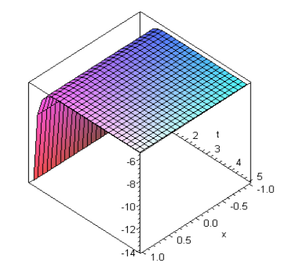
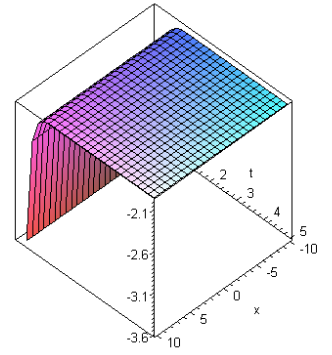
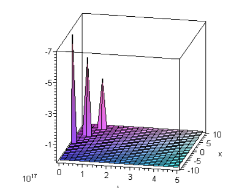
Figure 1. Solution of soliton h1(x, y) for k1=1, γ=1, λ=3, μ=1, k2=1.5
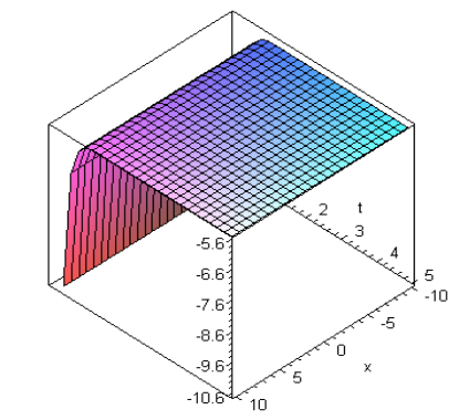
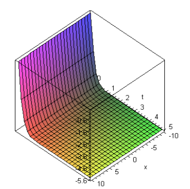
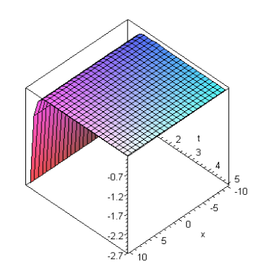
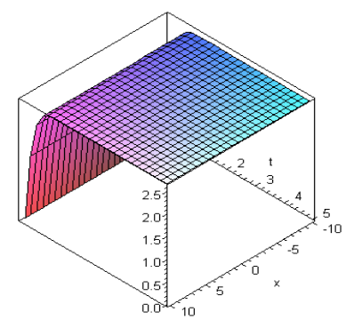
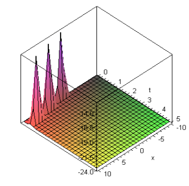
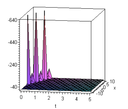
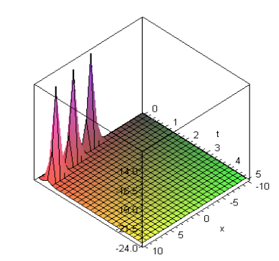
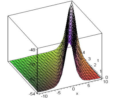
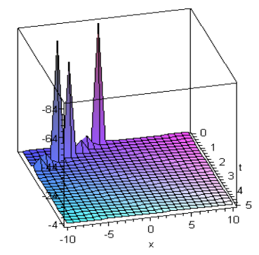
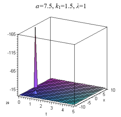
Through graphical demonstrations, we observe that the soliton is a wave that keeps its shape preserve after colliding by some other similar wave. By solving nonlinear evolution equations including the equation of foam drainage and the equation of 4th order evolution, we get required solitary wave solutions by using distinct values of random parameter. If the speed is positive, the solitary wave move in right direction and if the velocity is negative, it moves in left direction. The amplitude and velocities are controlled by parameters of various kind. Figures represent graphical illustration for different parameter values. Figure 1 describes a periodic wave solution by using parameters values as γ=1, λ=3 and μ=1, Figure 2 also describes a periodic wave solution by using parameters values as γ=1.5, λ=4 and μ=2. Similarly Figures from 1 to 11 demonstrate that periodic wave solution for different values of parameters. Figure 12 represents a solitary wave solution by using parameters values as λ=4 and μ=2. Figure 13 represents a solitary wave solution by using parameters values as λ=3 and μ=1. The soliton solution which are shown in Figures 12 to 15 and Figures 17 to 20 represents solitary wave solutions for different values of parameters like μ and λ. Figure 16 presents the peakon solution by using parameters values as μ=2 and λ=4. In all above discussed cases, we obtain identical solitary wave solutions for different values of parameters which absolutely show that the final solution is not always based on these parameters effectively. Therefore, we can consider random values of these parameters as input into our solutions. The results are obtained by using analytic technique (G'⁄G)-expansion method. Graphical representations reveal the accuracy of the proposed technique.
Figure 2. Solution of soliton h1(x, t) for k2=2.5, λ=4, γ=1.5, μ=2, k1=1
Figure 3. Solution of soliton h2(x, t) for λ=3, γ=1, μ=1
Figure 4. Solution of soliton h2(x, t) for γ=2, μ=2, λ=4
Figure 5. Solution of soliton h3(x, t) for μ=2, γ=2, λ=4
Figure 6. Solution of soliton h3(x, t) for λ=3, γ=2.5, μ=2
Figure 7. Solution of soliton h4(x, t) for k2=1.5, λ=3, γ=2.5, μ=2, k1=1
Figure 8. Solution of soliton h4(x, t) for μ=2, k2=2, k1=1.5, λ=2, γ=3
Figure 9. Solution of soliton h5(x, t) for λ=2, μ=2, γ=3
Figure 10. Solution of soliton h5(x, t) for μ=3, γ=3.5, λ=3
Figure 11. Solution of soliton h6(x, t) for μ=3, γ=3.5, λ=3
Figure 12. Solution of soliton m1(x, t) for λ=4, k1=2, b=2.5, k2=0.5, a=2.5, μ=2
Figure 13. Solution of soliton m1(x, t) for a=1.5, k1=1, μ=1, k2=1.5, λ=3, b=2
Figure 14. Solution of soliton m2(x, t) for a=1.5, λ=3, b=2, μ=1
Figure 15. Solution of soliton m2(x, t) for μ=2, λ=4, b=2.5
Figure 16. Solution of soliton m3(x, t) for a=2.5, μ=2, λ=4, b=2.5
Figure 17. Solution of Soliton m3(x, t) for λ=3, b=2, a=0.5, μ=2
Figure 18. Solution of soliton m4(x, t) for λ=2, k2=1.5, k1=1, μ=2, b=2, a=0.5
Figure 19. Solution of soliton m4(x, t) for μ=2, k2=2, b=1, a=7.5, k1=1.5, λ=1
Figure 20. Solution of Soliton m5(x, t) for λ=1, μ=2, b=1, $a$=7.5
The more general and also new useful exact solutions of NLEEs has been attained in this research paper via using the method of (G'⁄G)-expansion method. For this purpose, the equation of nonlinear foam drainage and the evolution equation of fourth order were considered. Through various values of parameters, we obtained the desired soliton solutions of different types. The exactness of the obtained results is guaranteed by using obtained solutions into the partial differential equation by using software Maple 18. The methodology of the proposed method is very simple, efficient and straightforward. It was observed that the method under consideration is reliable, effective and have lesser computational work. Precisely, this method is very reliable and widely applicable for obtaining exact solution of NLEEs. Computational work and the graphical illustration shows the validity of the given algorithm. Outcomes attained through this technique are straightforward and very encouraging to determine exact solutions of any kind of NLEEs. The graphical illustrations noticeably show the solitary solutions.
[1] Aslan, I. (2011). Exact and explicit solutions to some nonlinear evolution equations by utilizing the (G’/G)-expansion method. Applied Mathematics and Computation, 217(20): 8134-8139. http://dx.doi.org/10.1016/j.amc.2009.05.038
[2] Bekir, A. (2008). Application of the (G’/G)-expansion method for nonlinear evolution equations. Physics Letter A, 372(19): 3400–3406. http://dx.doi.org/10.1016/j.physleta.2008.01.057
[3] Feng, J., Li, W., Wan, Q. (2011). Using (G′/G)−expansion method to seek traveling wave solution of Kolmogorov-Petrovskii-Piskunov equation. Applied Mathematics and Computation, 217(12): 5860-5865. https://doi.org/10.1016/j.amc.2010.12.071
[4] Song, M., Ge, Y. (2010). Application of (G`/G)-expansion method to (3+1)-dimensional nonlinear evolution equations. Computers and Mathematics with Applications, 60(5): 1220-1227. https://doi.org/10.1016/j.camwa.2010.05.045
[5] Naher, H., Abdullah, F., Akbar, M.A. (2011). The (G′/G)−expansion method for abundant traveling wave solutions of Caudrey-Dodd-Gibbon equation. Mathematical Problems in Engineering, Article ID: 218216. https://doi.org/10.1155/2011/218216
[6] Ozis T., Aslan, I. (2010). Application of the (G′/G)−expansion method to Kawahara type equations using symbolic computation. Applied Mathematics and Computation, 216(8): 2360-2365. https://doi.org/10.1016/j.amc.2010.03.081
[7] Wang, M., Li X., Zhang, J. (2008). The (G′/G)−expansion method and traveling wave solutions of nonlinear evolution equations in mathematical physics. Physics Letter A, 372(4): 417-423. https://doi.org/10.1016/j.physleta.2007.07.051
[8] Zayed, E.M.E., Al-Joudi, S. (2010). Applications of an Extended (G′/G)−Expansion Method to Find Exact Solutions of Nonlinear PDEs in Mathematical Physics. Mathematical Problems in Engineering, Article ID: 768573. https://doi.org/10.1155/2010/768573
[9] Duranda M., Langevin, D. (2002). Physicochemical approach to the theory of foam drainage. The European Physical Journal E., 7: 35-44. https://doi.org/10.1140/epje/i200101092
[10] Naher, H., Abdullah, F.A., Akbar, M.A. (2013). Generalized and improved (G′/G)−expansion method for (3+1) dimensional modified KdV-Zakharov-Kuznetsev equation. Plos One, 8(5): e64618. http://dx.doi.org/10.1371/journal.pone.0064618
[11] Roshid, H., Akbar, M.A., Alam, M.N., Hoque, M.D., Rahman, N. (2014). New extended (G’/G)-expansion method to solve nonlinear evolution equation: the (3 + 1)-dimensional potential-YTSF equation. Springer Plus, 3: 122. https://doi.org/10.1186/2193-1801-3-122
[12] Chen, J., Li, B. (2012). Multiple (G`/G)-expansion method and its applications to nonlinear evolution equations in mathematical physics. Indian Academy of Sciences, 28(3): 375-388. https://doi.org/10.1007/s12043-011-0237-6
[13] Wang, M., Zhang, J., Li, X. (2008). Application of the (G'⁄G)-expansion to traveling wave solutions of the Broer-Kaup and the approximate long water wave equations. Applied Mathematics and Computation, 206(1): 321-326. https://doi.org/10.1016/j.amc.2008.08.045
[14] Aslan, I., Oz ̈is, T. (2009). Analytic study on two nonlinear evolution equations by using the (G`/G)-expansion method. Applied Mathematics and Computation, 209(2): 425-429. https://doi.org/10.1016/j.amc.2008.12.064
[15] Yang, X.J. (2017). A new integral transform operator for solving the heat-diffusion problem. Applied Mathematics Letters, 64: 193-197. https://doi.org/10.1016/j.aml.2016.09.011
[16] Yang, X.J. (2016). A New integral transform method for solving steady Heat transfer problem. Thermal Science, 20(suppl. 3): S639-S642. https://doi.org/10.2298/TSCI16S3639Y
[17] Yang, X.J., Tenreiro, J.A., Baleanu, D., Cattani, C. (2016). On exact traveling wave solutions for local fractional Korteweg-de Vries equation. Chaos, 26(8): 084312. http://dx.doi.org/10.1063/1.4960543
[18] Yang, X.J., Feng, G., Srivastava, H.M. (2017). Exact travelling wave solutions for the local fractional two-dimensional Burgers-type equations. Computers & Mathematics with Applications, 73(2): 203-210. http://dx.doi.org/10.1016/j.camwa.2016.11.012