Tohid Adibi* | Omid Adibi
OPEN ACCESS
In this paper, cavity flow is simulated numerically. Forced convection in different Reynolds numbers between 100 and 5000 is simulated. Different and complex thermal boundary conditions are applied and various parameters are calculated numerically. Up and down walls are in constant temperature and left and right walls are thermal insulation in the first thermal boundary condition. The Left and the down walls are in constant temperature and the temperature of the up and the right walls changes linearly in the second thermal boundary condition. For the third thermal boundary condition, the left and the down walls are in constant temperature and the temperature of the up and the right walls changes sinusoidally. For this purpose, a code is written in the FORTRAN software. Streamlines, isotherms, local and mean Nusselt number are obtained and shown in different figures and one table. Grid independence is surveyed and some obtained results are validated with other researchers' work. In these simulations, the Prandtl number is considered to be 0.71 because of the air’s Prandtl number. For time discretization, a fifth-order Runge-Kutta is used and for convective fluxes, the averaging scheme with fourth-order damping term is used.
cavity flow, forced convection, Reynolds number, complex boundary condition, Nusselt number
Numerical solution is an important way to solve mixed convection. A large number of numerical approaches have been created and developed for solving fluid problems. Many of the numerical methods for incompressible flows are mainly based on pressure corrections. The artificial compressibility of Chorin [1] is an alternative among the others. Where, by the help of pseudo-time derivative, the continuity and the momentum equations are coupled. Therefore, the hyperbolized governing equations admit the compressible flow methods. Natural and forced convections occur in several uses of science and technology. Natural and forced convections are mainly complex concerning several parameters such as the geometry and thermophysical characteristics of the fluid. Tmartnhad [2] carried out a numerical study of mixed convection in a trapezoidal cavity. The Navier–Stokes equations were solved using the semi-implicit method for pressure linked equations-consistent (SIMPLEC). Haeri and Shrimpton [3] used an implicit fictitious domain method where the entire domain was assumed to be incompressible. They used the SIMPLE algorithm with a collocated grid for free and forced convections. Srinivasa and Eswara [4] simulated unsteady free convection over an isothermal truncated cone with variable viscosity and Prandtl number. An implicit finite-difference scheme, along with quasilinearization, was used for solving coupled thermo-flow equations. Raji et al. [5] utilized SIMPLER for free convection in a square cavity. The convective fluxes were evaluated by a hybrid scheme in which the central differences are replaced by the first-order upwind scheme. Selimefendigil and Öztop [6] performed a numerical investigation of pulsating mixed convection in a multiply vented cavity for a range of Reynolds, Grashof, and Strouhal numbers. The convective fluxes in momentum and energy equations were solved by QUICK scheme, and SIMPLE method was used for velocity-pressure coupling. Sivasankaran et al. [7] carried out a numerical analysis of mixed convection in an inclined square cavity with different sizes and heater locations. The first-order upwind and second-order central schemes were used for the convective and diffusion fluxes, respectively. Billah et al. [8] analyzed mixed convection heat transfer in a lid-driven cavity and a heated circular hollow cylinder located at the center of the cavity. A Galerkin weighted residual finite element method was adopted to solve the governing equations.
Basak et al. [9] investigated natural convection in trapezoidal enclosures for uniformly heated bottom wall, linearly heated vertical wall(s) in the presence of the insulated top wall. Their method was a numerical method with penalty finite element method. Parametric studies for the wide range of Rayleigh numbers and Prandtl numbers with various tilt angles of side walls had been performed. Adibi and Razavi [10, 11] in two different works, simulated natural and forced convection in three benchmarks. Their benchmarks were squared cavity, flow between two parallel plates, and flow over a circular cylinder. They apllied a new characteristic-based scheme that was proposed by themselves. Adibi [12] extended their previous works [10, 11] to the three-dimensional flow with heat transfer. In this work, he added the momentum equation in the z-direction to other equations (continuity, x-momentum, y-momentum, and energy equations.). He obtained characteristics and hyper-surfaces. Also, he surveyed the influence of artificial compressibility parameter in his work. Bayat and Rahimi [13] solved convection heat transfer numerically. They solved Navier-Stokes equations with energy equation. They used simple algorithm.
Teschner et al. [14] simulated Navier-Stokes equations numerically. They used characteristic based schemes Rusanov’s Riemann solver to treat the convective term through a Godunov-type method. They applied artificial compressibility to connect the continuity equation to the momentum equations as our work. Adibi et al. [15] simulated mixed convection for various fluids by a characteristics-based scheme. Viscous terms were calculated by the averaging method. Alhumoud et al. [16] Simulated free convection by finite element method. The effects of the wall thermal conductivity, fluid and porous interfacial convective heat transfer factors and the Rayleigh number on the thermal behavior of the cavity were studied and analyzed. Mallikarjun et al. [17] simulated mixed convection numerically. Also, heat transfer factors such as Nusselt number, Sherwood number and skin friction parameters were obtained.
In this paper, forced convection in squared cavities is simulated numerically in different and complex thermal boundary conditions and different Reynolds numbers. Streamlines, isotherms, local Nusselt number and mean Nusselt number are obtained in this work. Also, the procedure of numerical method is explained in details.
The governing equations in dimensionless form for the two-dimensional incompressible viscous flow with heat transfer are
$\begin{align} & \frac{1}{\beta }\frac{\partial p}{\partial t}+\frac{\partial u}{\partial x}+\frac{\partial v}{\partial y}=0 \\ & \frac{\partial u}{\partial t}+u\frac{\partial u}{\partial x}+v\frac{\partial u}{\partial y}=-\frac{\partial p}{\partial x}+\frac{1}{\operatorname{Re}}(\frac{{{\partial }^{2}}u}{\partial {{x}^{2}}}+\frac{{{\partial }^{2}}u}{\partial {{y}^{2}}}), \\ & \frac{\partial v}{\partial t}+u\frac{\partial v}{\partial x}+v\frac{\partial v}{\partial y}=-\frac{Gr}{{{\operatorname{Re}}^{2}}}T \\ & -\frac{\partial p}{\partial y}+\frac{1}{\operatorname{Re}}(\frac{{{\partial }^{2}}v}{\partial {{x}^{2}}}+\frac{{{\partial }^{2}}v}{\partial {{y}^{2}}}), \\ & \frac{\partial T}{\partial t}+u\frac{\partial T}{\partial x}+v\frac{\partial T}{\partial y}=Ec(u\frac{\partial p}{\partial x}+v\frac{\partial p}{\partial y}) \\ & +\frac{1}{\operatorname{Re}\Pr }(\frac{{{\partial }^{2}}T}{\partial {{x}^{2}}}+\frac{{{\partial }^{2}}T}{\partial {{y}^{2}}})+\frac{Ec}{\operatorname{Re}}\Phi . \\ \end{align}$ (1)
In the free and the mixed convection, density is not constant. Hence the Boussinesq assumption is used. Where β is the artificial compressibility factor. Re, Pr, Ec, and Gr numbers are defined as:
$\begin{align} & \operatorname{Re}=\frac{{{\rho }_{ref}}{{u}_{ref}}{{L}_{ref}}}{\mu },\Pr =\frac{{{c}_{P}}\mu }{k}, \\ & Ec=\frac{u_{ref}^{2}}{{{c}_{P}}({{T}_{ref2}}-{{T}_{ref1}})}, \\ & Gr=\frac{{{\beta }_{ex}}g({{T}_{ref2}}-{{T}_{ref1}})L_{ref}^{3}}{{{\nu }^{2}}}. \\ \end{align}$ (2)
The Eq. (1) can be written in matrix form as
$\frac{\partial \mathbf{Q}}{\partial t}+\frac{\partial (\mathbf{F}-\mathbf{R})}{\partial x}+\frac{\partial (\mathbf{G}-\mathbf{S})}{\partial y}~=\mathbf{H}.$ (3)
In the above equation, ‘Q,’ ‘F,’ ‘R’ , ‘G’ , ‘S’ , and ‘H’ are
$\begin{align} & \mathbf{Q}=\left[ \begin{matrix} \begin{matrix} p \\ u \\\end{matrix} \\ \begin{matrix} v \\ T \\\end{matrix} \\\end{matrix} \right]~,\,\text{ }\mathbf{F}=\left[ \begin{matrix} \beta u \\ p+{{u}^{2}} \\ uv \\ (T-Ec\text{ }p)u \\\end{matrix} \right] \\ & \mathbf{G}=~\,\,\left[ \begin{matrix} \beta v \\ uv \\ p+{{v}^{2}} \\ (T-Ec\text{ }p)v \\\end{matrix} \right]\,,\,\,\mathbf{R}=\frac{1}{\operatorname{Re}}\left[ \begin{matrix} 0 \\ \frac{\partial u}{\partial x} \\ \frac{\partial v}{\partial x} \\ \frac{1}{\Pr }\frac{\partial T}{\partial x} \\\end{matrix} \right],\text{ }\,\,\,\,\, \\ & \mathbf{S}=\frac{1}{\operatorname{Re}}\left[ \begin{matrix} 0 \\ \frac{\partial u}{\partial y} \\ \frac{\partial v}{\partial y} \\ \frac{1}{\Pr }\frac{\partial T}{\partial y} \\\end{matrix} \right],\,\,\,\,\,\,\,\,\,\,\,\mathbf{H}=\left[ \begin{matrix} 0 \\ 0 \\ \frac{Gr}{{{\operatorname{Re}}^{2}}}T \\ \frac{Ec}{\operatorname{Re}}\Phi \\\end{matrix} \right]. \\ \end{align}$ (4)
After some mathematics calculation and using the green theorem, the governing equations for the two-dimensional incompressible viscous thermo-flow in the finite-volume form can be expressed as
$\frac{\partial }{\partial t}\iint{\mathbf{Q}dA}+\oint{((\mathbf{F}-\mathbf{R})dy-(\mathbf{G}-\mathbf{R})dx)}=\iint{\mathbf{H}dA},$ (5)
In the above equations ‘F’ and ‘G’ are the convective fluxes and ‘R’ and ‘S’ are the viscous fluxes and ‘H’ is the source.
3.1. Numerical scheme
After discretization of the Eq. (5), one has
${{A}_{ij}}\frac{\partial {{\mathbf{Q}}_{ijk}}}{\partial t}=\left[ \sum\limits_{m=1}^{4}{{{(({{\mathbf{F}}_{ijk}}-{{\mathbf{R}}_{ijk}})\Delta y-({{\mathbf{G}}_{ijk}}-{{\mathbf{S}}_{ijk}})\Delta x)}_{m}}}-{{A}_{ij}}{{\mathbf{H}}_{ijk}} \right],\,\,\,\,k=1,2,3,4$ (6)
For time discretization, one can use the backward method. So
$\frac{\partial {{\mathbf{Q}}_{ijk}}}{\partial t}=\frac{\mathbf{Q}_{ijk}^{n}-\mathbf{Q}_{ijk}^{n-1}}{\Delta t}=\frac{1}{{{A}_{ij}}}\left[ \sum\limits_{m=1}^{4}{{{(({{\mathbf{F}}_{ijk}}-{{\mathbf{R}}_{ijk}})\Delta y-({{\mathbf{G}}_{ijk}}-{{\mathbf{S}}_{ijk}})\Delta x)}_{m}}}-{{A}_{ij}}{{\mathbf{H}}_{ijk}} \right]n-1,\,\,\,\,k=1,2,3,4\,\,\,\,\,\,\Rightarrow \,\,\,\,\,\,{{\mathbf{Q}}^{n}}=\Delta t*\Psi ({{\mathbf{Q}}^{n-1}})+{{\mathbf{Q}}^{n-1}}$ (7)
where, $\Psi\left(Q^{n-1}\right)$ is a function of the velocities, the pressure, and the temperature in the last step. In this paper, for time discretization, a fifth-order Runge-Kutta is utilized which reads.
$\begin{align} & {{\mathbf{\Phi }}^{(0)}}={{\mathbf{Q}}^{n-1}} \\ & {{\mathbf{\Phi }}^{(p)}}={{\alpha }_{p}}\Delta t*\Psi ({{\mathbf{\Phi }}^{p-1}})+{{\mathbf{\Phi }}^{p-1}},\,\, \\ & {{\alpha }_{p}}=\frac{1}{4},\text{ }\frac{1}{6},\text{ }\frac{3}{8},\text{ }\frac{1}{2},1,\text{ }p=1,2,...,5. \\ & {{\mathbf{Q}}^{(n)}}={{\mathbf{\Phi }}^{(5)}} \\ \end{align}$ (8)
In this type of the Runge-Kutta method, the values in each step of the Runge-Kutta method don’t need to be saved. To calculate the convective fluxes, the averaging scheme is used. In this scheme, the convective fluxes are determined by
$\begin{align} & {{\lambda }^{*}}=({{\lambda }_{i,j}}+\,{{\lambda }_{i+1,j}})/2\,,\,\,\,\,\,\,\,\,\,\,\,\, \\ & \lambda =p,\,\,\,u,\,\,\,v,\,\,\,and\,\,T. \\ \end{align}$ (9)
The flux averaging method is an unstable method in various condition, so the fourth-order damping term is used as
$D=-\varepsilon {{(\Delta x)}^{4}}\frac{{{\partial }^{4}}u}{\partial {{x}^{4}}}$ (10)
where, ‘D’ is the fourth-order damping term, and ‘ε’ is the damping coefficient. This term is added explicitly to the right-hand side of Eq. (6). A negative sign is needed to produce positive dissipation. This forth-order dissipation is approximated by a central differences discretization as
${{(\Delta x)}^{4}}\frac{{{\partial }^{4}}u}{\partial {{x}^{4}}}={{u}_{i-2}}-4{{u}_{i-1}}+6{{u}_{i}}-4{{u}_{i+1}}+{{u}_{i+2}}$ (11)
The viscous fluxes demand the computation of derivatives at the cell faces. For this purpose, the following procedure on the secondary cell is done (the green theorem is used again to convert double integral to line integral).
${{\left. \frac{\partial \eta }{\partial x} \right|}_{AB}}=\frac{1}{S}\iint\limits_{S}{\frac{\partial \eta }{\partial x}\,ds=\frac{1}{S}}\oint{\eta dy}=\frac{1}{S}\sum\limits_{k=1}^{4}{\eta \Delta {{y}_{k}}},\,\,\,\,\,\,\,\,\eta =u,v,T.$ (12)
In the above equation, k=1 to 4 are corresponding to the sides of the secondary cells. Now, the velocities and the temperature on the sides of the secondary cells must be determined. The corresponding variables are found by averaging method. For example values on the first side are calculated by
${{\eta }_{k=1}}=0.5*({{\eta }_{A}}+{{\eta }_{i,j}})=0.5*\left[ 0.25*\left( {{\eta }_{i,j}}+{{\eta }_{i,j+1}}+{{\eta }_{i+1,j}}+{{\eta }_{i+1,j+1}} \right)+{{\eta }_{i,j}} \right]$ (13)
3.2 Boundary conditions
In the walls, the no-slip condition is applied to determine the velocities and the temperature, and the pressure is extrapolated from the interior domain. The second-order extrapolation is used as
${{p}_{s}}=1.5{{p}_{i,1}}-0.5{{p}_{i,2}}$ (14)
In this paper, the cavity flow is simulated in three different thermal boundary conditions. For the velocities, the boundary conditions are displayed in Eq. (15).
uup=1, udown=0, uleft=0, right=0. (15)
As mentioned, for temperature, three different boundary conditions are simulated in this paper. The first thermal boundary conditions are
$\begin{align} & {{T}_{up}}=1,\,\,{{T}_{Down}}=0,\,\,\, \\ & {{\left[ \frac{dT}{dx} \right]}_{for\,\,left\,\,and\,\,right\,\,walls}}=0 \\\end{align}$ (16)
Above equations show that the up wall is hot and the down wall is cold. Also, those equations display that left and right walls are isolated. The second thermal boundary conditions are
${{T}_{Up}}=x,\,\,{{T}_{Down}}=0,\,\,\,{{T}_{left}}=0,\,\,{{T}_{Right}}=y.$ (17)
Above equations show that the down and the left walls are cold and the temperature of the right and up walls increases linearly from cold to hot. The third thermal boundary conditions are
$\begin{align} & {{T}_{Up}}=\sin (\pi x),\,\,{{T}_{Down}}=0,\,\,\,\, \\ & {{T}_{left}}=0,\,\,{{T}_{Right}}=\sin (\pi y). \\\end{align}$ (18)
Above equations show that the down and the left walls are cold and the temperature of the right and up walls increases linearly from cold to hot. The third thermal boundary conditions are sinusoid.
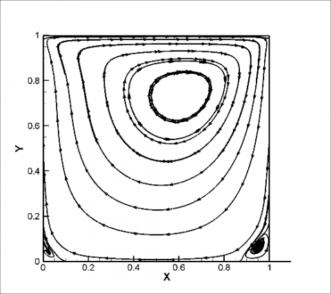
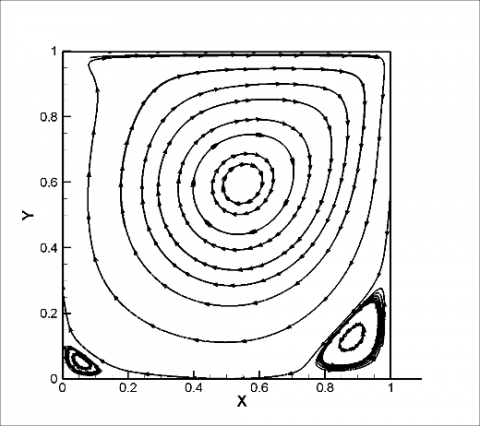
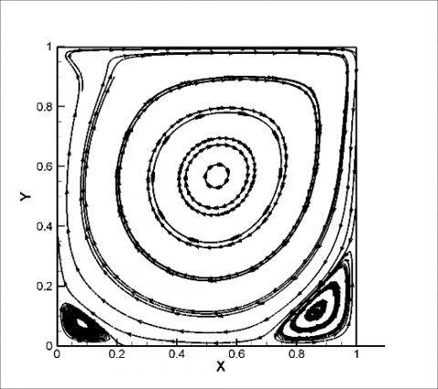
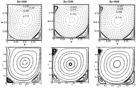
Simulations are done in different Reynolds numbers. Results are displayed in different form as streamlines, isotherms, and Nusselt number. Streamlines in different Reynolds number are shown in Figure 1. In this paper, the Grashof number is considered zero, hence, streamlines pattern does not depend on the thermal boundary conditions. In all conditions, there are one main vortex and two secondary vortices. These secondary vortices become larger as the Reynolds number increases.
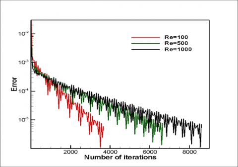
Error at every step is calculated by
$Error=\sqrt{\frac{\sum{\sum{{{\left( V_{i,j}^{n+1}-V_{i,j}^{n} \right)}^{2}}}}}{N*M}}$ (19)
Convergence history is displayed in Figure 2.
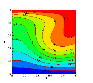
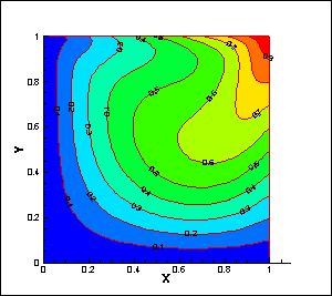
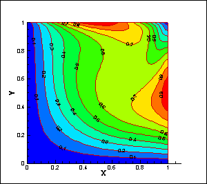
Isotherm lines pattern depend on thermal boundary conditions. Isotherms are shown at different Reynolds numbers in Figure 3 at the first thermal boundary condition. In low Reynolds numbers, convection is not so important especially in the down part of the cavity and heat is transferred by conduction, as a result isotherms are almost parallel. But in high Reynolds numbers, heat is transferred by fluid motion, and forced convection is strong. The local Nusselt number is one of the important dimensionless numbers in flow with heat transfer. To calculate the Nusselt number, this procedure is done.
$\begin{align} & {q}''=h\Delta T=k\frac{\partial T}{\partial y},\,\,\,\,\, \\ & Nu=\frac{hL}{k}=\frac{kL\frac{\partial T}{\partial y}}{k\Delta T}=\frac{L\frac{\partial T}{\partial y}}{\Delta T} \\\end{align}$ (20)
The above equation in dimensionless form is
$Nu=\frac{\partial T}{\partial y}$ (21)
After discretization one has
$N{{u}_{i}}=\frac{{{T}_{i,2}}-{{T}_{i,1}}}{{{y}_{i,2}}-{{y}_{i,1}}}$ (22)
Re=100
Re=500
Re=1000
Figure 1. Streamlines in different Reynolds numbers at Gr=0, Pr= 0.71
Figure 2. Convergence history in different Reynolds numbers with Gr=0, Pr= 0.71
Re=100
Re=500
Re=1000
Figure 3. Isotherm lines at different Reynolds numbers in the first thermal boundary condition
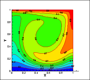
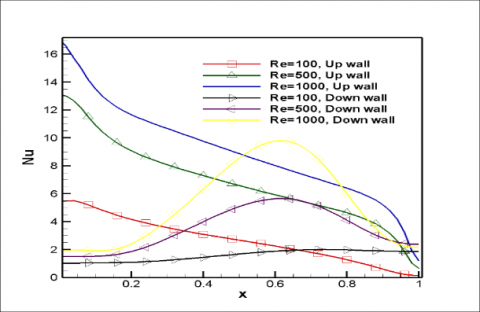
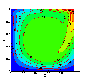
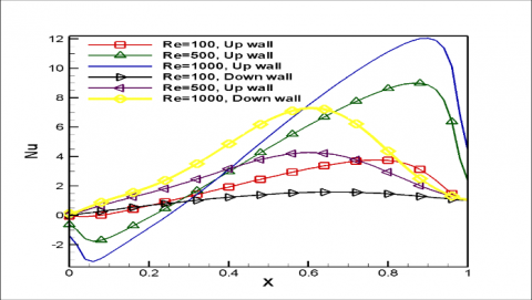
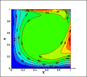
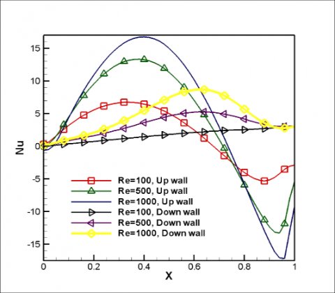
The Nusselt number for the up and the down wall in the different Reynolds number are displayed in Figure 4. According to the results, the local Nusselt number for the up wall is more than the local Nusselt number for the down wall because the velocity near the up wall is more than the velocity near the down wall. For up wall, local Nusselt number decreases throughout the up wall because the thickness of the boundary layer increases along the up wall, but about the down wall, the variation of local Nusselt number is complex. Different parameters affect the Nusselt number magnitude. As a result, the local Nusselt number is maximum at one point on the down wall. Also, the results display that the local Nusselt number is more at higher Reynolds number as it is expected. In this part, the thermal boundary conditions are changed according to the equation (17) in the written code. Novel simulation is done, and new results are obtained. The isotherms are displayed in Figure 5 at the different Reynolds numbers. In the low Reynolds numbers, conduction is more important and in the high Reynolds numbers, convection is more important in heat transfer. In the high Reynolds number, most parts of the cavity are in the medium temperature, and only the parts near walls are different. In other words, the thickness of the boundary layer is low in the high Reynolds numbers.
Figure 4. Local Nusselt number for up and down walls in different Reynolds number at Gr=0, Pr= 0.71 in the first thermal boundary condition
Re=100
Re=500
Re=1000
Figure 5. Isotherm lines in the different Reynolds numbers in the second thermal boundary condition
The local Nusselt numbers for the up and the down walls are shown in Figure 6. Results show that the Nusselt number is maximum in the one points of the up and the down walls. For the up wall in the high Reynolds numbers, the Nusselt number is negative for the first part of the wall. This shows that the heat transfer direction is from the fluid to the wall because of the new thermal boundary conditions. In new boundary conditions, the temperature of the up wall changes from zero at the first point of the up wall to one at the endpoint of the up wall. Hence, the temperature of the fluid near the up wall in the first part is more than the temperature of the up wall at that part. Therefore, heat transfers from the fluid to the up wall and the Nusselt number is negative at that part.
Figure 6. Local Nusselt number for the up and the down walls in the different Reynolds number at Gr=0, Pr= 0.71 in the second thermal boundary condition
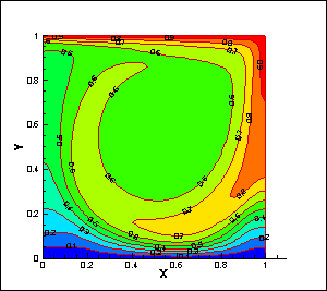
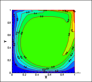
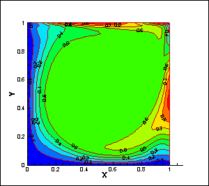
Simulations are done for the third boundary conditions in this part. The isotherms are displayed in Figure 7 in the different Reynolds numbers. In the low Reynolds numbers, conduction is more important and in the high Reynolds numbers, convection is more important in heat transfer The Nusselt numbers for the up and the down walls are shown in Figure 8. Results show that the local Nuselt number variation is complex because the thermal boundary conditions are complicated specially for the up wall. In these thermal boudary conditions, the local Nusselt number is higher than the previous thermal boundary conditions. For the up wall, the local Nusselt number is negative in the end part of the wall because the temperature of this part is less than the temperature of the near fluid. As a result, the heat transfer from the fluid to the wall therefore, the local Nusselt number is negative. In this section, the mean Nusselt number is calculated for all three thermal boundary conditions. To obtain the mean Nusselt number, this procedure is done.
$\overline{Nu}=\frac{1}{L}\int_{0}^{L}{Nu\,}dx$ (23)
The mean Nusselt number in dimensionless form is
$\overline{Nu}=\int_{0}^{1}{Nu\,}dx$ (24)
After discretization one has
$\overline{Nu}=\frac{1}{m}\sum\limits_{i=1}^{m}{N{{u}_{i}}}\,$ (25)
Re=100
Re=500
Re=1000
Figure 7. Isotherm lines in the different Reynolds numbers in the third thermal boundary condition
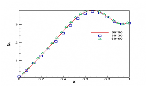
Obtained mean Nusselt number is displayed in table 1. The mean Nusselt number is increased when the Reynolds number rises. The mean Nusselt number is more for the up wall in all conditions except one condition. The mean Nusselt number is more for the down wall in the third thermal boundary condition at Re=1000 because in this state Nusselt number is negative in some parts of the wall and is positive in other parts and because the mean Nusselt number is average of two sections, its magnitude is low. In other words, if the mean Nusselt number were the average of the absolute value of Nusselt numbers in positive and negative parts, its magnitude would be larger. Grid independence is surveyed and is Shown in Figure 9. In this figure, the local Nusselt number is shown for the down wall in different grids at Re=300. The number of cells in this grid are 30×30, 50×50, and 70×70. To verify the results, they are validated with Cheng and Lui [18] results. So streamlines in different Reynolds numbers are calculated then they are shown and compared with those of Cheng and Lui in Figure 10.
Figure 8. Local Nusselt number for up and down walls in different Reynolds number at Gr=0, Pr= 0.71 in the third thermal boundary condition
Figure 9. Nusselt number variation for down wall in three different grids (30×30, 50×50, and 60 ×60) at Re=300, Gr=0, Pr=0.7
In this paper, the forced convection is simulated in cavity flow in three complex thermal boundary conditions. The streamlines and the isotherms are obtained and are interpreted. Results show that there are one main vortex and two secondary vortices in the different Reynolds numbers. The secondary vortices become larger when the Reynolds number rises. Also, the local Nusselt numbers and the mean Nusselt numbers are calculated for the up and the down walls. Results show that the local Nusselt numbers and the mean Nusselt numbers are more in the high Reynolds numbers. In the complex thermal boundary conditions, the local Nusselt number of some parts of the up wall becomes negative. In these states, heat transfers from fluid to the up wall because fluid temperature, near that part of the wall, is more than wall temperature. Most of the obtained figures have one or more extremums. Creation and growth of boundary layers at walls are seen in most of the results.
Table 1. Mean Nusselt number for three thermal boundary conditions
|
|
|
Re=100 |
Re=500 |
Re=1000 |
|
Down wall |
The first thermal boundary condition |
1.5642 |
3.4740 |
5.2474 |
|
The second thermal boundary condition |
1.0974 |
2.4957 |
3.7951 |
|
|
The third thermal boundary condition |
1.6816 |
3.2222 |
4.6294 |
|
|
Up wall |
The first thermal boundary condition |
2.7275 |
6.8468 |
9.0651 |
|
The second thermal boundary condition |
2.0055 |
3.9272 |
4.7983 |
|
|
The third thermal boundary condition |
1.7640 |
3.5429 |
4.5629 |
Figure 10. Comparisons of the streamlines in the different Re at Gr=0, Pr= 0.71
[1] Chorin, A.J. (1997). A numerical method for solving incompressible viscous flow problems. Journal of Computational Physics, 135(2): 118-125. http://dx.doi.org/10.1006/jcph.1997.5716
[2] Tmartnhad, I., El Alami, M., Najam, M., Oubarra, A. (2008). Numerical investigation on mixed convection flow in a trapezoidal cavity heated from below. Energy Conversion and Management, 49(11): 3205-3210. http://dx.doi.org/10.1016/j.enconman.2008.05.017
[3] Haeri, S., Shrimpton, J.S. (2013). A new implicit fictitious domain method for the simulation of flow in complex geometries with heat transfer. Journal of Computational Physics, 237: 21-45. http://dx.doi.org/10.1016/j.jcp.2012.11.050
[4] Srinivasa, A.H., Eswara, A.T. (2013). Unsteady free convection flow and heat transfer from an isothermal truncated cone with variable viscosity. International Journal of Heat and Mass Transfer, 57(1): 411-420. http://dx.doi.org/10.1016/j.ijheatmasstransfer.2012.10.054
[5] Raji, A., Hasnaoui, M., Naïmi, M., Slimani, K., Ouazzani, M.T. (2012). Effect of the subdivision of an obstacle on the natural convection heat transfer in a square cavity. Computers & Fluids, 68: 1-15. http://dx.doi.org/10.1016/j.compfluid.2012.07.014
[6] Selimefendigil, F., Öztop, H.F. (2014). Numerical investigation and dynamical analysis of mixed convection in a vented cavity with pulsating flow. Computers & Fluids, 91: 57-67. http://dx.doi.org/10.1016/j.compfluid.2013.11.033
[7] Sivasankaran, S., Sivakumar, V., Hussein, A.K. (2013). Numerical study on mixed convection in an inclined lid-driven cavity with discrete heating. International Communications in Heat and Mass Transfer, 46: 112-125. http://dx.doi.org/10.1016/j.icheatmasstransfer.2013.05.022
[8] Billah, M.M., Rahman, M.M., Sharif, U.M., Rahim, N.A., Saidur, R., Hasanuzzaman, M. (2011). Numerical analysis of fluid flow due to mixed convection in a lid-driven cavity having a heated circular hollow cylinder. International Communications in Heat and Mass Transfer, 38(8): 1093-1103. http://dx.doi.org/10.1016/j.icheatmasstransfer.2011.05.018
[9] Basak, T., Roy, S., Singh, A., Pandey, B.D. (2009). Natural convection flow simulation for various angles in a trapezoidal enclosure with linearly heated side wall(s). International Journal of Heat and Mass Transfer, 52(19-20): 4413-4425. http://dx.doi.org/10.1016/j.ijheatmasstransfer.2009.03.057
[10] Adibi, T., Razavi, S.E. (2015). A new-characteristic approach for incompressible thermo-flow in cartesian and noncartesian grids. International Journal for Numerical Methods in Fluids, 79(8): 371-393. http://dx.doi.org/10.1002/fld.4053
[11] Razavi, S.E., Adibi, T. (2016). A novel multidimensional characteristic modeling of incompressible convective heat transfer. Journal of Applied Fluid Mechanics, 9: 1135-1146. http://dx.doi.org/10.18869/acadpub.jafm.68.228.24295
[12] Adibi, T. (2018). Three-dimensional characteristic approach for incompressible thermo-flows and influence of artificial compressibility parameter. Journal of Computational & Applied Research in Mechanical Engineering (JCARME), 8(2): 223-234. http://dx.doi.org/10.22061/jcarme.2018.2032.1178
[13] Bayat, R., Rahimi, A.B. (2017). Numerical solution of N-S equations in the case of unsteady axisymmetric stagnation-point flow on a vertical circular cylinder. International Journal of Thermal Sciences, 118: 386-396. https://doi.org/10.1016/j.ijthermalsci.2017.05.007
[14] Teschner, T.R., Könözsy, L., Jenkins, K. (2018). Predicting non-linear flow phenomena through different characteristics-based schemes. Aerospace, 5(1): 22. https://doi.org/10.3390/aerospace5010022
[15] Adibi, T., Adibi, O., Razavi, S.E. (2019). A characteristic-based solution of forced and free convection in closed domains with emphasis on various fluids. International Journal of Engineering, 32(11): 1679-1685. http://dx.doi.org/10.5829/ije.2019.32.11b.20
[16] Alhumoud, J.M. (2019). Non-equilibrium natural convection flow through a porous medium. Mathematical Modelling of Engineering Problems, 6(2): 163-169. https://doi.org/10.18280/mmep.060202
[17] Mallikarjun, P., Murthy, R.V., Mahabaleshwar, U.S., Lorenzini, G. (2019). Numerical study of mixed convective flow of a couple stress fluid in a vertical channel with first order chemical reaction and heat generation/absorption. Mathematical Modelling of Engineering Problems, 6(2): 175-182. https://doi.org/10.18280/mmep.060204
[18] Cheng, T.S., Liu, W.H. (2010). Effect of temperature gradient orientation on the characteristics of mixed convection flow in a lid-driven square cavity. Computers & Fluids, 39(6): 965-978. http://dx.doi.org/10.1016/j.compfluid.2010.01.009