Mohammad Sanjeed Hasan | Rabindra Nath Mondal* | Giulio Lorenzini
OPEN ACCESS
In this paper, a numerical study on centrifugal instability with convective heat transfer through a curved square duct is presented by using a spectral method, and covering a wide range of the Dean number $\left( 0<Dn\le 5000 \right)$ for a tightly coiled square duct of curvature 0.5 The outer and bottom walls of the duct are heated while cooling from the inner and the ceiling. The main objective of this study is to expose combined effects of centrifugal and buoyancy forces on fluid flows through a curved channel. For this purpose, solution structure of the steady solutions is obtained first. As a result, four branches of symmetric/asymmetric steady solutions are obtained. Linear stability of the steady solutions is then investigated. It is found that only the first branch is linearly stable while the other branches are linearly unstable. Unsteady flow behavior, obtained by time evolution calculations, shows that the steady-state flow turns into chaotic flow via periodic and multi-periodic flows, if Dn is increased. Typical contours of secondary flow pattern, stream-wise velocity distribution and temperature profiles are obtained at several values of Dn and it is found that the flow consists of asymmetric two- to four-vortex solutions. The present study shows that convective heat transfer is significantly enhanced by the secondary flow; and the chaotic flow, which occurs at large Dn’s, enhances heat transfer more effectively than the steady-state or periodic solutions. Finally, a comparison between the numerical and experimental investigations has been made, and it is found that there is a good agreement between the numerical and experimental investigations.
curved square duct, secondary flow, steady solution, unsteady solution, heat transfer
Fluid flow through curved passages is a common occurrence in a vast range of industrial applications, such as in gas turbine blades, air conditioning, heat exchangers and rocket engine coolant passages. In a curved passage, centrifugal forces are developed in the flow due to channel curvature causing a counter rotating vortex motion applied on the axial flow through the passage. This creates characteristic spiraling fluid flow in the curved passage known as secondary flow. At a certain critical flow condition and beyond, additional pairs of counter rotating vortices appear on the outer concave wall of curved fluid passages. This flow condition is referred to as Dean’s Hydrodynamic Instability and the additional vortices are known as Dean vortices, in recognition of the pioneering work in this field by Dean [1]. The readers are referred to Ito [2], Joseph et al. [3] and Mondal et al. [4] for some outstanding reviews on curved duct flows.
Centrifugal forces are very efficient mechanism to destablize flows. Among generic cases one can cite the Dean flow between two curved walls close to each other, the Taylor–Couette flow between two rotating cylinders and the Görtler flow over a concave wall [5]. In all these cases, the geometry is infinite in one direction perpendicular to centrifugal forces, and the basic flow is two-dimensional. However, an important circumstance of the flow through a curved duct is the bifurcation of the flow because various types of steady solutions are existed for the presence of centrifugal force which is affected by the curvature of the duct. It has already seen that many authors have been presented the bifurcation structure both numerically and experimentally for various types of duct such as helically coiled ducts [3, 6], rectangular ducts [7] and oval [8]. Wang et al. [9] performed both bifurcation and stability for coiled ducts, where the same phenomena was studied by Yamamoto et al. [10] for helical tube. Chandratilleke et al. [11-13] reported extensive parametric study examining the effects of curvature ratio and aspect ratio as well as the wall heat flux. The validation of their numerical work had been performed against their experimental data [11, 12]. Their numerical method, that was effectively a two-dimensional formulation, used toroidal coordinate system and utilized a stream function approach with dynamic similarity in axial direction. Mondal et al. [14] presented numerical simulation of the flow characteristics and found substantial results where the secondary flow was affected by the convective heat transfer. Recently, Mondal et al. [15] discussed the onset of secondary vortices with a large range of Grashof numbers.
Time-dependent behavior of the curved duct flow was analyzed both numerically and experimentally by Arnal et al. [16], where the solution structure of the unsteady solution was first introduced by Yanase and Nishiyama [17]. Time evolution calculations of the Nusselt number were performed for a wide range of Dean number by Mondal et al. [18]. Yanase et al. [19] also obtained the unsteady solutions for aspect ratio 2 and a flow characteristics is found (steady state $\rightarrow$ periodic $\rightarrow$ chaotic). Wang and Liu [20] performed numerical as well as experimental investigations of periodic oscillations for the fully developed flow in a curved square duct. Flow visualization in the range of Dean numbers from 50 to 500 was conducted in their experiment. Flow transitions in the curved square duct for various types of curvatures were also investigated by Mondal et al. [21]. The fluctuation of heat between the steady solutions and the unsteady solutions are also showed by them. Later Mondal et al. [14] discussed that the fluid flow undergoes various types of instabilities in the unstable region. However, solution structure as well as transient behavior of the unsteady solution is not yet resolved for the flow through a strongly curved square duct with differentially heated sidewalls, which motivated the present study to fill up this gap.
A remarkable characteristic of the flow through a curved duct is to enhance heat transfer to the fluid from two differentially heated sidewalls. However, experimental investigations of heat transfer in curved duct flows are limited because of the difficulties associated with the measurement of fluid temperature profile, while corresponding numerical calculations are reported by many authors. Chandratilleke et al. [22] presented a numerical investigation to examine the secondary vortex motion and heat transfer process in fluid flow through curved rectangular ducts of aspect ratios 1 to 6. The study formulated an improved simulation model based on 3-dimensional vortex structures for describing secondary flow and its thermal characteristics. Wu et al. [23] performed numerical study of the secondary flow characteristics in a curved square duct by using spectral method, where the walls of the duct except the outer wall rotate around the centre of curvature and an azimuthal pressure gradient was imposed. The secondary flow characteristics in a curved square duct were investigated experimentally by using visualization method by Yamamoto et al. [24]. Recently, Razavi et al. [25] investigated flow characteristics, heat transfer and entropy generation in a curved duct by using control volume method. Very recently, Li et al. [26] conducted a combined experimental and numerical study on 3D flow development in a curved rectangular duct with varying curvature. Effects of curvature, Reynolds number and aspect ratio on hydrodynamic instability were discussed in that paper to accurately predict the core of secondary base vortices.
In the present paper, we propose to study fully developed 2D flow through a tightly coiled square duct of strong curvature. The main objective of this study is to find out solution structure of the steady solutions and to investigate unsteady flow behavior with effects of secondary vortices on convective heat transfer. The study formulates and verifies a novel approach for computational scheme in identifying onset of hydrodynamic instability in a curved passage reflected by Dean vortex generation.
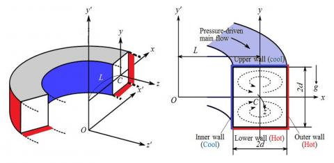
Consider a hydro-dynamically and thermally fully developed two-dimensional (2D) flow of viscous incompressible fluid through a curved square duct. The physical geometry is shown in Figure 1, where the x′ and y′ axes are taken in the horizontal and vertical directions respectively, and z′ in the flow direction. It is assumed that the outer and bottom walls of the duct are heated while cooling from the inner and the ceiling walls. It is assumed that the flow is driven by a constant pressure gradient G along the centre-line of the duct as shown in Figure 1. The dimensional variables are made non-dimensional by using the representative length d and the representative velocity ${{U}_{0}}=\nu /d$, where $\nu$ is the kinematic viscosity of the fluid.
Figure 1. Non-rotating co-ordinate system of the curved duct
By assumption of symmetric flow, stream functions for the cross-sectional velocities have the following form
$\left. \begin{align} & u=\frac{1}{r}\frac{\partial \psi }{\partial y}=\frac{1}{1+\delta x}\frac{\partial \psi }{\partial y} \\ & v=-\frac{1}{r}\frac{\partial \psi }{\partial x}=-\frac{1}{1+\delta x}\frac{\partial \psi }{\partial x} \\\end{align} \right\}$ (1)
Equation (1) satisfies the continuity equation. Now stream-wise velocity$\left( w \right)$, cross-sectional stream function$\left( \psi \right)$ and energy/temperature $\left( T \right)$ are defined based on the Navier-Stokes equation as follows:
$\left( 1+\delta x \right)\frac{\partial w}{\partial t}=Dn-\frac{\partial (w,\psi )}{\partial (x,y)}+\frac{{{\delta }^{2}}w}{1+\delta x}+(1+\delta x){{\Delta }_{2}}w-\frac{\delta }{1+\delta x}\frac{\partial \psi }{\partial y}w+\delta \frac{\partial w}{\partial x}$ (2)
$\begin{align} & \left( {{\Delta }_{2}}-\frac{\delta }{1+\delta x}\frac{\partial }{\partial x} \right)\stackrel{\scriptscriptstyle\to}{\leftarrow}\frac{\partial \psi }{\partial \text{ }t}=-\frac{1}{(1+\delta x)}\frac{\partial \text{ }({{\Delta }_{2}}\psi ,\psi )}{\partial \text{ }(x,y)}++w\frac{\partial w}{\partial y} \\ & \frac{\delta }{{{(1+\delta x)}^{2}}}\left[ \frac{\partial \psi }{\partial y}\left( 2{{\Delta }_{2}}\psi -\frac{3\delta }{1+\delta x}\frac{\partial \psi }{\partial x}+\frac{{{\partial }^{2}}\psi }{\partial {{x}^{2}}} \right)-\frac{\partial \psi }{\partial x}\frac{{{\partial }^{2}}\psi }{\partial x\partial y} \right] \\ & +\frac{\delta }{{{(1+\delta x)}^{2}}}\times \left[ 3\delta \frac{{{\partial }^{2}}\psi }{\partial {{x}^{2}}}-\frac{3{{\delta }^{2}}}{1+\delta x}\frac{\partial \psi }{\partial x} \right]-\frac{2\delta }{1+\delta x}\frac{\partial }{\partial x}{{\Delta }_{2}}\psi \\ & +{{\Delta }_{2}}^{2}\psi -Gr(1+\delta x)\frac{\partial T}{\partial x} \\\end{align}$ (3)
$\frac{\partial T}{\partial t}+\frac{1}{(1+\delta x)}\frac{\partial (T,\,\psi )}{\partial (x\,,y)}=\frac{1}{\Pr }\left( {{\Delta }_{2}}T+\frac{\delta }{1+\delta x}\frac{\partial T}{\partial x} \right)$ (4)
The non-dimensional parameters $Dn$, the Dean number; $Gr$, the Grashof number and $\Pr $, the Prandtl number, which appear in equation (2) to (4) are defined as
$Dn=\frac{G{{d}^{3}}}{\mu \upsilon }\sqrt{\frac{2d}{L}},\text{ }Gr=\frac{\beta g\Delta T{{d}^{3}}}{{{\upsilon }^{2}}},\stackrel{\scriptscriptstyle\to}{\leftarrow}\Pr =\frac{\upsilon }{\kappa }$ (5)
The no-slip rigid boundary conditions for $w$and $\psi $are taken as
$w\left( \pm 1,y \right)=w\left( x,\pm 1 \right)=\psi \left( \pm 1,y \right)=\psi \left( x,\pm 1 \right)=\frac{\partial \psi }{\partial x}\left( \pm 1,y \right)=\frac{\partial \psi }{\partial y}\left( x,\pm 1 \right)$ (6)
and temperature $T$ is assumed to be constant on the walls as
$T\left( x,1 \right)=1,\text{ T}\left( \text{x,-1} \right)=-1,\text{ T}\left( \pm \text{1,y} \right)=y$ (7)
3.1 Method of numerical calculations
In order to get numerical solution, spectral method is used (Gottlieb and Orazag [27]). By this method the variables are expanded in the series of the function consisting of Chebychev polynomials. The expansion functions ${{\varphi }_{n}}\left( x \right)$ and ${{\psi }_{n}}\left( x \right)$ are expressed as
$\left. \begin{align} & {{\varphi }_{n}}\left( x \right)=\left( 1-{{x}^{2}} \right){{C}_{n}}\left( x \right) \\ & {{\psi }_{n}}\left( x \right)={{\left( 1-{{x}^{2}} \right)}^{2}}{{C}_{n}}\left( x \right) \\\end{align} \right\}$ (8)
where, ${{C}_{n}}\left( x \right)=\cos \left( n{{\cos }^{-1}}\left( x \right) \right)$ is the n-th order Chebyshev polynomial. $w\left( x,y,t \right)$, $\psi \left( x,y,t \right)$ and $T\left( x,y,t \right)$ are expanded in terms of ${{\varphi }_{n}}\left( x \right)$ and ${{\psi }_{n}}\left( x \right)$ as
$\left. \begin{matrix} w(x,y,t)=\sum\limits_{m=0}^{M}{\sum\limits_{n=0}^{N}{{{w}_{m\,n}}\,(t)\,{{\phi }_{m}}\,(x)\,{{\phi }_{n}}\,(y)\,}} \\ \psi (x,y,t)=\sum\limits_{m=0}^{M}{\sum\limits_{n=0}^{N}{{{\psi }_{m\,n}}\,(t)\,{{\psi }_{m}}\,(x)\,{{\psi }_{n}}\,(y)}} \\ T(x,y,t)=\sum\limits_{m=0}^{M}{\sum\limits_{n=0}^{N}{{{T}_{m\,n}}\,(t)\,{{\varphi }_{m}}\,(x)\,{{\varphi }_{n}}(y)}-y} \\\end{matrix} \right\}$ (9)
Here, M and N are the truncation numbers in the x- and y-directions respectively, and ${{w}_{mn}}$, ${{\psi }_{mn}}$ and ${{T}_{mn}}$are the coefficients of expansion. To obtain steady solution $\overline{w}\left( x,y \right)$, $\overline{\psi }\left( x,y \right)$and $\overline{T}\left( x,y \right)$, the expansion series (9) is then substituted into the basic equations (2) - (4), and the collocation method is applied.
Linear stability of the steady solutions is investigated against only two-dimensional perturbations (z-independent). For this purpose, the eigenvalue problem is solved by application of the function expansion method together with collocation method to the linearized equations for the perturbation of $\overline{w}\left( x,y \right)$, $\overline{\psi }\left( x,y \right)$ and $\overline{T}\left( x,y \right)$. It is supposed that the time dependence of the perturbation is${{e}^{\sigma t}}$, where$\sigma ={{\sigma }_{r}}+i{{\sigma }_{i}}$. If all the real parts${{\sigma }_{r}}$of the eigenvalue $\sigma $ are negative, the steady solution is linearly stable, but if there exist at least one positive real part, it is linearly unstable. In the unstable region, the perturbation grows monotonically for${{\sigma }_{i}}=0$and oscillatory for${{\sigma }_{i}}\ne 0$. Finally, in order to calculate the unsteady solutions, the Crank-Nicolson and Adams-Bashforth methods together with the function expansion (9) and the collocation methods are applied to equations (2) - (4).
3.2 Resistance coefficient
The resistance coefficient $\lambda$ is used as the representative quantity of the flow state. It is also called the hydraulic resistance coefficient, and is generally used in fluids engineering, defined as
$\frac{P_{1}^{*}-P_{2}^{*}}{\Delta {{z}^{*}}}=\frac{\lambda }{d_{h}^{*}}\frac{1}{2}\rho {{\left\langle {{w}^{*}} \right\rangle }^{2}}$ (10)
where quantities with an asterisk denote dimensional ones, $d_{h}^{*}$ is the hydraulic diameter, $\left\langle {} \right\rangle $ stands for the mean over the cross section of the duct, $\rho $is the density is the density, and $P_{1}^{*}$ and $P_{2}^{*}$are the pressure at the upstream and downstream positions of the duct respectively. The mean axial velocity $\left\langle {{w}^{*}} \right\rangle $ is calculated by
$\left\langle {{w}^{*}} \right\rangle =\frac{\nu }{4\sqrt{2\delta }d}\int_{-1}^{1}{dx\int_{-1}^{1}{{\bar{w}}}}\left( x,y,t \right)dy$ (11)
Since $\frac{P_{1}^{*}-P_{2}^{*}}{\Delta {{z}^{*}}}=G$, $\lambda $ is related to the mean non-dimensional axial velocity $\left\langle w \right\rangle =\sqrt{2\delta }d\left\langle {{w}^{*}} \right\rangle /\nu $as
$\lambda =\frac{4\sqrt{2\delta }Dn}{{{\left\langle w \right\rangle }^{2}}}$ (12)
It should be remarked that$\lambda \propto D{{n}^{-1}}$in the limit of $Dn\to 0$with $\delta $ kept constant, since $\left\langle w \right\rangle \propto Dn$ in this limit.
3.3 Numerical accuracy
Here, the validation of the numerical study has been tested with changing the truncation numbers. As the paper is based on curved square duct, we therefore consider N = M, where M and N are the grid sizes along the horizontal and vertical axis respectively. Table 1 shows the values of the resistance coefficient $\left( \lambda \right)$and the axial flow $\left( w \right)$ at the origin for various values of M and N. As seen in Table 1, the numerical accuracy is attained if we take M = 24 and N = 24. Therefore, throughout this investigation, we use the truncation number M = 24 and N = 24.
Table 1. The values of $\lambda $ and $w\left( 0,0 \right)$ for various M and N at $Dn=100$, $Gr=500$ and $\delta =0.5$
|
M |
N |
$\lambda $ |
$w\left( 0,0 \right)$ |
|
16 |
16 |
0.634661134821 |
341.43833392975 |
|
18 |
18 |
0.6347971982070 |
341.704442189362 |
|
20 |
20 |
0.6347909128331 |
341.931772761516 |
|
22 |
22 |
0.6347702723961 |
342.094338341262 |
|
24 |
24 |
0.6347763788143 |
342.220108367290 |
|
26 |
26 |
0.6347764048319 |
342.321432031774 |
4.1 Steady solutions and linear stability analysis
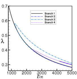
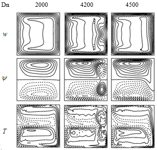
In this study, solution structure of the steady solutions has been investigated by Newton-Raphson iteration method, and pattern variation of secondary flows on various branches of steady solutions has been discussed. After an extensive survey over the range of the parameters, four branches of asymmetric steady solutions are obtained over the Dean number$\text{0}Dn\le 5\text{000}$for$Gr=100$. A bifurcation diagram of steady solutions is shown in Figure 2(a) using $\lambda $, the representative quantity of the solutions. The four steady solution branches are named the first steady solution branch (Branch 1, solid line), the second steady solution branch (Branch 2, dashed dot dot line), the third steady solution branch (Branch 3, dashed dot line), the fourth steady solution branch (Branch 4, dotted line), respectively. The solution branches are obtained by the path continuation technique with various initial guesses and are distinguished by the nature and the number of secondary flow vortices appearing in the cross section of the duct. In this regard, it should be noted that this type of solution structure was observed by Mondal et al. [4] for the isothermal flow through a curved square duct of curvature 0. 2797. Figure 3 shows typical contours of stream-wise velocity, secondary flow patterns and isotherm on various branches of steady solutions at different Dean numbers. It is found that the branches consist of asymmetric two- to four-vortex solutions; two-vortex at moderate Dn’s while two- and four-vortex at large Dn’s. Linear stability of the steady solutions shows that among four branches of steady solutions, only the first branch is linearly stable while the other branches are linearly unstable. The first branch is linearly stable for $0<Dn\le 4410.14$and unstable otherwise. Thus a saddle-node bifurcation occurs at $Dn=4410.14$.
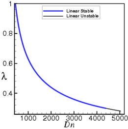
As seen in Table 2, the perturbation grows oscillatorily $\left( {{\sigma }_{i}}\ne 0 \right)$ for$Dn\ge 4410.14$. Therefore, a Hopf bifurcation occurs at$Dn=4410.14$. The stability region on the first branch is shown by a blue solid line in Fig. 2(b), where linearly unstable region by thin solid black line. In this regard, it should be remarked that this kind of bifurcation has also been obtained by Winters [28] for the isothermal flow through non-rotating curved ducts with square and rectangular cross section of small curvature $(\delta =0.02).$
In this study, contours of temperature profiles show that the streamlines of the heat flow are uniformly distributed to all parts of the contour transferring heat from the heated walls to the fluid, and the contribution of the buoyancy and pressure on secondary flows significantly change and increase the number of secondary vortices. It is clearly evident that heating the bottom and outer wall causes the temperature contours to become asymmetrical in comparison to isothermal cases. This essentially arises from the interaction between the heating-induced buoyancy force and the centrifugal force that drives secondary vortices. In this regard, it should be noted that the centrifugal force due to the duct curvature creates two effects; it generates a positive radial fluid pressure field in the duct cross section and induces a lateral fluid motion driven from inner wall towards the outer wall. This lateral fluid motion occurs against the radial pressure field generated by the centrifugal effect and is superimposed on the axial flow to create the secondary vortex flow structure. As the flow through the curved duct is increased, the lateral fluid motion becomes stronger and the radial pressure field is intensified. In the vicinity of the outer wall, the combined action of adverse radial pressure field and viscous effects slows down the lateral fluid motion and forms a stagnant flow region. Beyond a certain critical value of Dn, the radial pressure gradient becomes sufficiently strong to reverse the flow direction of the lateral fluid flow. A weak local flow re-circulation is then established creating an additional pair of vortices in the stagnant region near the outer wall. This flow situation is known as Dean’s hydrodynamic instability.
(a)
(b)
Figure 2. (a) Solution structure of steady solutions for $0<Dn\le 5000,\text{ }\delta \text{=0}\text{.5}$, (b) Linear stability of the 1st steady solution branch
Figure 3. Flow patterns on the steady solution branches for $\delta =0.5$ at various values of $Dn$
Table 2. Stability analysis for the first steady solution branch for$\delta =0.5,\text{ Gr =100}$ and $\text{0Dn}\le \text{5000}$
|
Dn |
$\lambda $ |
${{\sigma }_{r}}$ |
${{\sigma }_{i}}$ |
|
100 500 |
0.95301468192 0.92801497890 |
-0.5835 -1.4232 |
0 0 |
|
1000 |
0.62940475033 |
-1.6886 |
0 |
|
2000 |
0.43985239666 |
-2.0121 |
0 |
|
3000 |
0.35922535134 |
-2.2368 |
0 |
|
4000 |
0.31290872468 |
-2.4153 |
0 |
|
4410.14 |
0.29882585018 |
-1.84´10-4 |
-8.79´101 |
|
4410.15 |
0.29882553444 |
3.87´10-5 |
-8.79´101 |
|
4500 |
0.29607508513 |
1.9523 |
-9.04´101 |
|
5000 |
0.28206939463 |
1.22´101 |
1.04´102 |
4.2 Unsteady solutions by time-evolution calculation
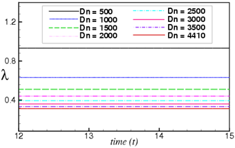
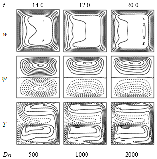
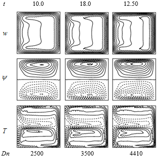
In order to investigate non-linear behavior of the unsteady solutions, time evolution calculations are performed. First, time evolutions of $\lambda $ are performed for $500\le Dn\le 4410$ as shown in Figure 4. It is found that the unsteady flow is a steady-state solution for all values of Dn in the range, which agrees well with the linear stability results presented in Sec. 4.1. Since the flow is steady-state, a single contour of each of the stream-wise velocity, secondary flow and isotherm is shown in Figure 5 for $500\le Dn\le 4410$. As seen in Fig. 5, the unsteady flow is an asymmetric two-vortex solution. The study shows that the streamlines of the secondary flow consist of two opposite vortices; one is an outward flow (anticlockwise direction) shown by solid line and the other one inward flow (clockwise direction) shown by dotted lines. The flow is accelerated due to combined action of the centrifugal and buoyancy forces; centrifugal force is created due to the motion through a curved channel while buoyancy forces because of the thermal gradient.
Figure 4. Unsteady solution for $\delta =0.5$and $500\le Dn\le 4410$
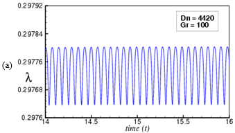
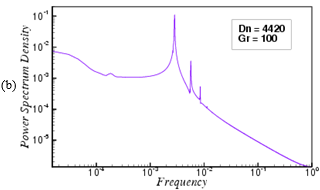
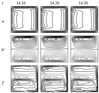
Then we increased Dean number and predicted unsteady solution at Dn=4420. Figure 6(a) shows time-history result for Dn=4420, which shows that the unsteady flow is a periodic oscillating flow at Dn=4420. This periodic oscillation is well justified by sketching the power spectrum density using log-log scale as shown in 6(b). Figure 6(b) shows that a fundamental frequency with large amplitude and its harmonics are seen which justifies that the unsteady flow presented in Figure 6(a) is periodic. To observe the flow patterns, as time proceeds, we obtain typical contours of secondary flow, stream-wise velocity distribution and isotherms for Dn=4420 as shown in Figure 7. Figure 7 shows that the time-dependent flow at Dn=4420 is an asymmetric two-vortex solution. As seen in Figures. 4 and 6, the transition from steady-state to periodic oscillation occurs between Dn=4410 and Dn=4420, which agrees with the linear stability result.
Figure 5. Streamlines of stream-wise velocity (top), secondary flow (middle) and isotherm (bottom) for$Dn=500,\text{ 1000, 2000, 2500, 3500, }4410$
Figure 6. (a) Unsteady solution, (b) Power spectrum density for$Dn=4420$and $\delta \text{= 0}\text{.5}\text{.}$
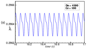
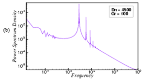
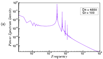
Then we then proceeded to perform time history of$\lambda $for$Dn=4500$, which is a multi-periodic solution as shown in Figure 8(a). To justify the flow characteristics, power spectrum density is calculated for$Dn=4500$ using log-log scale as shown in Figure 8(b). Figure 8(b) shows that fundamental frequency and its harmonics are seen but not any sub-harmonics of the fundamental frequency are available, which justifies that the unsteady flow presented in Figure 8(a) is periodic for$Dn=4500$ rather than multi-periodic. To observe vortex generation and temperature distribution for the periodic oscillation at $Dn=4500$, stream-wise velocity, streamlines and isotherms are obtained as shown in Figure 9 for $Dn=4500$. Figure 9 shows that the flow is an asymmetric two-vortex solution for$Dn=4500$. In fact, the periodic oscillation, which is observed in the present study, is a traveling wave solution advancing in the downstream direction which is well justified in the investigation by Yanase et al. [29] for a three-dimensional travelling wave solutions as an appearance of 2D periodic oscillation. If Dn is increased a little, for example$Dn=4550$, the periodic flow turns into multi-periodic flow. Figure 10(a) shows time-evolution of $\lambda $for$Dn=4550$, which shows that the time-dependent flow is a multi-periodic flow for$Dn=4550$and it is well justified by obtaining power spectrum density using log-log scale as shown in Fig. 10(b). Streamlines of stream-wise velocity, secondary flow velocity and isotherm for $Dn=4550$ are shown in Figure 11. As seen in Figure 11, the time-dependent flow is a two-vortex solution for$Dn=4550$. From Figures 8(a) and 10(a), it is concluded that the transition from periodic to multi-periodic oscillation lakes place between Dn=4500 and Dn=4550.
Figure 7. Streamlines of stream-wise velocity (top), secondary flow (middle) and isotherm (bottom) for $Dn=4420$and $\delta \text{=0}\text{.5}\text{.}$
Figure 8. (a) Unsteady solution, (b) Power spectrum density for$Dn=4500$and $\delta \text{= 0}\text{.5}\text{.}$
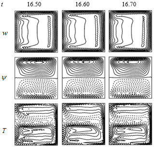
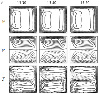
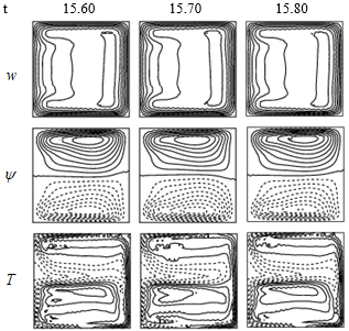
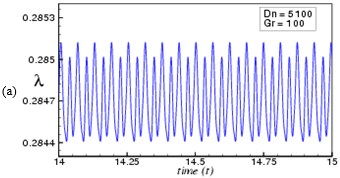
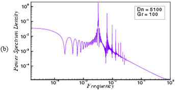
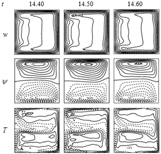
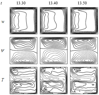
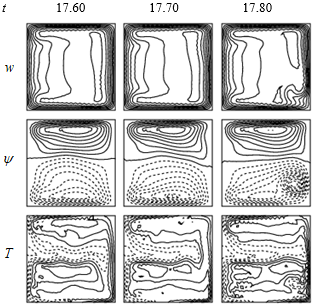
Then we seek for the transition from multi-periodic to chaotic oscillation. For this purpose we increased the Dean number and predicted unsteady solutions. Figures 12(a) and 14(a) respectively show time-dependent flows for Dn=5100 and Dn=5150. It is found that the time-dependent flow at Dn=5100 (Figure 12(a)) is a multi-periodic flow while at Dn=5150 (Figure 14(a)) a chaotic solution. These multi-periodic or chaotic oscillations are well justified by drawing the power spectrum density of the unsteady solutions as shown in Figures 12(b) and Figure 14(b) for Dn=5100 and Dn=5150 respectively. As seen in Fig. 12(b), not only the line spectrum of the fundamental frequency and its harmonics but other line spectrum with different frequencies are seen, which indicates that the flow at Dn=5100 is multi-periodic. Figure 14(b), on the other hand, shows that there appears continuous line spectrum of different frequencies, which confirms that the flow presented in Figure 14(a) is chaotic. This sort of flow behavior has been called transitional chaos (Mondal et al., [4]) because the multi-periodic flow becomes chaotic through this process, where the line spectra with low frequencies turn into the continuous spectrum. Thus the transition from multi-periodic to chaotic oscillation happens between Dn=5100 and Dn=5150. Streamlines of stream-wise velocity, secondary flow velocity and isotherm for Dn=5100 and Dn=5150 are shown in Figures 13 and 15 respectively. It is found that unsteady flows at Dn=5100 and Dn=5150 are asymmetric two-vortex solution. If the Dean number is increased further, for example, Dn=5500, the unsteady flow remains chaotic as shown in Figure 16(a) for time-evolution result and in Figure 16(b) for power spectrum density. As seen in Figure 16(b), the line spectra with smaller frequencies that were observed in Figure 12(b) for multi-periodic oscillation completely disappear and continuous line spectrum overlap each other in a non-linear pattern so that the unsteady flow presented in Figure 16(a) is fully chaotic. This type of chaotic oscillation is termed as strong chaos (Mondal et al., [4]). It should be noted that, the occurrence of the chaotic state, as presented in the present study, is related with destabilization of the periodic or quasi-periodic solutions which reminds us the case of Lorenz attractor [30]. It may be possible that the transition in the present study is caused by a similar mechanism as that of Ruelle-Takens scenario [31] in the laminar flow. Then we obtained streamlines of stream-wise velocity, secondary flow pattern and isotherm for Dn=5500 as shown in Figure 17. It is found that the chaotic flow oscillates irregularly in the asymmetric two-vortex solution. It is found that axial flow is shifted near the outer wall as the pressure gradient force becomes strong. Temperature distribution is found to be consistent with the secondary vortices and a strong interaction is observed between the heating-induced buoyancy force and the centrifugal instability, which stimulates fluid mixing and thus results in thermal enhancement in the flow. In this study, it is found that secondary flow enhances heat transfer in the flow and as the flow becomes chaotic heat transfer occurs substantially from the heated walls to the fluid.
Figure 9. Streamlines of stream-wise velocity (top), secondary flow (middle) and isotherm (bottom) for$Dn=4500,\text{ }\delta \text{=0}\text{.5}\text{.}$
By the time-evolution calculations with their power spectrum analysis, it is found that stable steady solutions are realized for$0<Dn\le 4410$, periodic solution for$4420\le Dn\le 4500$, multi-periodic for $4550\le Dn\le 5100$ and chaotic for$Dn\ge 5150$. Therefore, the transition from steady-state to periodic flow occurs between Dn=4410 and Dn=4420. Linear stability analysis indicates that the stable steady solutions exist for $0<Dn\le 4410.14$ while unstable for$Dn\ge 4410.15$. Therefore, the results of the linear stability analysis and those of the time-evolution calculations are consistent, so that the realizability for the steady and periodic solutions is perfectly dominated by the nature of the bifurcation diagram.
Figure 10. (a) Unsteady solution, (b) Power spectrum density forand$\delta \text{= 0}\text{.5}\text{.}$
Figure 11. Streamlines of stream-wise velocity (top), secondary flow (middle) and isotherm (bottom) for$Dn=4550,\text{ }\delta \text{=0}\text{.5}\text{.}$
Figure 12. (a) Unsteady solution, (b) Power spectrum density for$Dn=5100$and $\delta \text{= 0}\text{.5}\text{.}$
Figure 13. Streamlines of stream-wise velocity (top), secondary flow (middle) and isotherm (bottom) for$Dn=5100,\text{ }\delta \text{=0}\text{.5}\text{.}$
Figure 14. (a) Unsteady solution, (b) Power spectrum density for$Dn=5150$and $\delta \text{= 0}\text{.5}\text{.}$
Figure 15. Streamlines of stream-wise velocity (top), secondary flow (middle) and isotherm (bottom) for$Dn=5150,\text{ }\delta \text{=0}\text{.5}\text{.}$
Figure 16. (a) Unsteady solution, (b) Power spectrum density for$Dn=5500$and $\delta \text{= 0}\text{.5}\text{.}$
Figure 17. Streamlines of stream-wise velocity (top), secondary flow (middle) and isotherm (bottom) for$Dn=5500,\text{ }\delta \text{=0}\text{.5}\text{.}$
4.3 Convective heat transfer
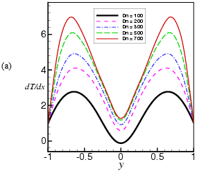
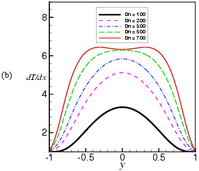
To study the phenomena for the convective heat transfer from the heated walls to the fluid, temperature gradient on the cooling and heated sidewalls are also calculated as shown in Figure 18. As seen in Figure 18(a), the temperature gradient $\frac{\partial T}{\partial x}$on the cooling sidewall declines in the central part near the line $y=0$ as Dn increases. This is mainly be fallen by the advective heat generation of the Dean flow in the outward direction around $y=0$ due to the centrifugal force. In the same figure, it is also shown that $\frac{\partial T}{\partial x}$ limit to soar up in the regions other than the central region for$Dn=100$. This happens due to advection of the secondary flow in the inward direction, which is an opposite flow of the outward secondary flow in the central region. As seen in Figure 18(b), $\frac{\partial T}{\partial x}$ raises monotonically over the whole region as Dn goes up from 100. This is actually caused as the secondary flow enhances enough $\frac{\partial T}{\partial x}$ not only in the central region but in other areas as well, if Dn is increased. Thus as seen in Figure 18, the tendency of increasing the temperature gradient at the heated wall is much significant than that in the cooling wall, which can be explained by the fact that heat transfer occurs frequently from the heated wall to the fluid as Dn increases.
Figure 18. Temperature Gradient (T.G). (a) cooling wall, (b) heating wall
4.4 Validation of the numerical result
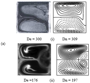
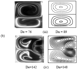
Here, the validation of our numerical result has been shown with the experimental data. By using visualization method, Wang and Yang [32] conducted experimental investigations of the flow through a stationary curved square duct of curvature $\delta =0.03$ while Chandratilleke [11] conducted that for $\delta =0.032$(Fig. 19(a)). On the contrary, Yamamoto et al. (2006) performed experimental investigations of the flow through a rotating curved square duct of curvature $\delta =0.03$for positive rotation of the duct at the Taylor number Tr=150 (Figure 13(b)). For comparison, as shown in Figure 19, we obtain the flow pattern for the same curvature as Wang and Yang [32], Chandratilleke [11] and Yamamoto et al. [24] used, and we see that our numerical results have a good agreement with the experimental investigations.
Figure 19. Experimental vs. numerical results for curved square duct flow. (a) Stationary duct. Left: Experimental result by (i) Wang and Yang [32] and (ii) Chandratilleke [11], right: numerical result by the authors. (b) Rotating duct. Left: Experimental result by Yamamoto et al. [24], right: numerical result by the authors (right)
The present paper investigates numerical simulation of two-dimensional laminar flow of viscous incompressible fluid streaming through a tightly coiled square duct of strong curvature $\left( \delta =0.5 \right)$. The outer and bottom walls of the duct are heated while cooling from the inner and ceiling. First, solution structure of the steady solutions is investigated by using path using continuation technique. As a result, we obtained four branches of symmetric/asymmetric steady solutions comprising with two- to four-vortex solutions. Linear stability analysis shows that only the first branch is linearly stable in the region $0<Dn\le 4410.14$ while the other branches are completely linearly unstable. Time-evolution results, justified by power spectrum density of the solutions, show that the unsteady flow undergoes in the scenario “Steady$\to $periodic$\to $multi-periodic$\to $chaotic”, if Dn is increased. The transition process from periodic to multi-periodic and then to chaotic state is well determined by power spectrum analysis, which may correspond to the destabilization of travelling waves in the curved channel flow like that of Tollmien-Schlichting waves in the boundary layer. The study shows that bifurcation diagram perfectly dominate the realizability of the steady and periodic solutions. The present study also shows that secondary flow enhances heat transfer in the flow particularly when Dean vortices emerge at the outer concave wall and if the flow is multi-periodic and then chaotic, as Dn increases, heat transfer occurs significantly. Finally, our numerical results have been compared with the experimental investigations obtained by some authors, and it is found that there is a good agreement between the numerical and experimental investigations.
|
Dn |
Dean number |
|
|
Gr |
Grashof number |
|
|
Pr |
Prandtl number |
|
|
a |
Aspect ratio |
|
|
L |
Radius of the curvature |
|
|
x |
Horizontal axis |
|
|
y |
Vertical axis |
|
|
z |
Axis in the direction of the main flow |
|
|
u |
Velocity components in the $x-$direction |
|
|
v |
Velocity components in the $y-$direction |
|
|
w |
Velocity components in the $z-$direction |
|
|
T |
Temperature |
|
|
t |
Time |
|
|
Greek symbols |
||
|
$\delta $ |
Curvature of the duct |
|
|
$\rho $ |
Density |
|
|
$\lambda $ |
Resistance coefficient |
|
|
$\mu $ |
Viscosity |
|
|
$\kappa $ |
Thermal diffusivity |
|
|
$\upsilon $ |
Kinematic viscosity |
|
|
$\psi $ |
Sectional stream function |
|
[1] Dean, W.R. (1927). Note on the motion of fluid in a curved pipe. Philos Mag., 4: 208-23. https://.doi.org/10.1112/S0025579300001947
[2] Ito, H. (1987). Flow in curved pipes. JSME International Journal, 30: 543-52. https://doi.org/10.1299/jsme1987.30.543
[3] Joseph, B., Smith, E.P., Adler, R.J. (1975). Numerical treatment of laminar flow in helically coiled tubes of square cross section. AIChE Journal, 21: 965-974. https://doi.org/10.1002/aic.690210519
[4] Mondal, R.N., Kaga, Y., Hyakutake, T., Yanase, S. (2007). Unsteady solutions and the bifurcation diagram for the flow through a curved square duct. Fluids Dynamics Research, 39: 413-446. https://doi.org/10.1016/j.fluiddyn.2006.10.001
[5] Drazin, P.G., Reid, W.H. (1981). Hydrodynamic Stability. Cambridge University Press, Cambridge. https://doi.org/10.1017/S0022112082212614
[6] Daskopoulos, P., Lenhoff, A.M. (1989). Flow in curved ducts: Bifurcation structure for stationary ducts. Journal of Fluid Mechanics, 20: 125-148. https://doi.org/10.1017/S0022112089001400
[7] Shantini, W., Nandakumar, K. (1986). Bifurcation phenomena of generalized Newtonian fluids in curved rectangular ducts. Journal of Non-Newtonian Fluid Mechanics, 22: 35-60. https://doi.org/10.1016/0377-0257(86)80003-9
[8] Kao, H.C. (1992). Some aspects of bifurcation structure of laminar flow in curved ducts. Journal of Fluid Mechanics, 243: 519-539. https://doi.org/10.1017/S0022112092002805
[9] Wang, L., Pang, O., Cheng, L. (2005). Bifurcation and stability of forced convection in tightly coiled ducts: Multiplicity. Chaos, Solitons and Fractals, 26: 337-352. https://doi.org/10.1016/S0169-5983(97)00032-4
[10] Yamamoto, K., Yanase, S., Jiang, R. (1998). Stability of flow in helical tube. Fluid Dynamics Research, 22: 153-70. https://doi.org/10.1016/S0169-5983(97)00032-4
[11] Chandratilleke, T.T. (2001). Secondary flow characteristics and convective heat transfer in a curved rectangular duct with external heating. Proceedings of 5th World Conference on Experimental Heat Transfer, Fluid Mechanics and Thermodynamics [ExHFT-5], Thessaloniki, Greece 1: 573-578.
[12] Chandratilleke, T.T. (1998). Performance enhancement of a heat exchanger using secondary flow effects. Proceedings of 2nd Pacific-Asia Conference in Mechanical Engineering, Manila, Philippines.
[13] Chandratilleke, T.T., Nursubiyakto. (2002). Numerical prediction of secondary flow and convective heat transfer in externally heated curved rectangular ducts. Int. J. Thermal Sciences 42: 187–198. https://doi.org/10.1016/S1290-0729(02)00018-2
[14] Mondal, R.N., Uddin, M.S., Yanase, S. (2010). Numerical prediction of non-isothermal flow through a curved square duct. Int. J. Fluid Mech. Research, 37: 85-99. https://doi.org/10.1615/InterJFluidMechRes.v37.i1.60
[15] Mondal, R.N., Watanabe, T., Hossain, M.A., Yanase, S. (2017). Vortex-structure and unsteady solutions with convective heat transfer trough a curved duct. Journal of Thermophysics and Heat Transfer, 31: 243-254. https://doi.org/10.2514/1.T4913
[16] Arnal, M.P., Goering, D.J., Humphrey, J.A.C. (1992). Unsteady laminar flow developing in a curved duct. Int. J. Heat Fluid Flow, 13: 347-57. https://doi.org/10.1016/0142-727X(92)90005-T
[17] Yanase, S., Nishiyama, K. (1988). On the bifurcation of laminar flows through a curved rectangular tube. J. Phys Soc. Japan, 57: 3790-3795. https://doi.org/10.1143/JPSJ.57.3790
[18] Mondal, R.N., Islam, M.S, Hossain, S.M.T. (2009). Flow instability through a Curved Duct with Square Cross Section. Journal of Bangladesh Mathematical Society, 29: 71-85. https://doi.org/10.3329/ganit.v29i0.8517
[19] Yanase, S., Mondal, R.N., Kaga, Y. (2005). Numerical study of non-isothermal flow with convective heat transfer in a curved rectangular duct. Int. J. Thermal Sci., 44: 1047-1060. https://doi.org/10.1016/j.ijthermalsci.2005.03.013
[20] Wang, L.Q., Liu, F. (2007). Forced convection tightly coiled ducts: Bifurcation in a high Dean number region. International Journal of Non-linear Mechanics, 42: 1018-1034. https://doi.org/10.1016/j.ijnonlinmec.2007.05.005
[21] Mondal, R.N., Kaga, Y., Hyakutake, T., Yanase, S. (2006). Effects of curvature and convective heat transfer in curved square duct flows. Trans. ASME, Journal of Fluids Engineering, 128: 1013-1022. https://doi.org/10.1115/1.2236131
[22] Chandratilleke, T.T., Nadim, N., Narayanaswamy, R. (2012). Vortex structure-based analysis of laminar flow behavior and thermal characteristics in curved ducts. Int. J. Thermal Sci., 59: 75-86. https://doi.org/10.1016/j.ijthermalsci.2012.04.014
[23] Wu, X.Y., Lai, S.D., Yamamoto, K., Yanase, S. (2013). Numerical analysis of the flow in a curved duct. Advanced Materials Research, 706-708: 1450-1453. https://doi.org/10.4028/www.scientific.net/AMR.706-708.1450
[24] Yamamoto, K., Wu, X., Kazuo, N., Yasutaka, H. (2006). Visualization of Taylor-Dean flow in a curved duct of square cross-section. J. Fluid dynamics research, 38: 1-18. https://doi.org/10.1016/j.fluiddyn.2005.09.002
[25] Razavi, R., Soltanipour, S.E., Choupani, P. (2015). Second law analysis of laminar forced convection in a rotating curved duct. Thermal Science, 19(1): 95-107. https://doi.org/10.2298/TSCI120606034R
[26] Li, Y., Wang, X., Yuan, S., Tan, S.K. (2016). Flow development in curved rectangular ducts with continuously varying curvature. Experimental Thermal and Fluid Science, 75: 1-15. https://doi.org/10.1016/j.expthermflusci.2016.01.012
[27] Gottlieb, D., Orazag, S.A. (1977). Numerical Analysis of Spectral Methods. Society of Industrial and Applied Mathematics, Philadelphia, USA. https://trove.nla.gov.au/version/13786328
[28] Winters, K.H. (1987). A bifurcation study of laminar flow in a curved tube of rectangular cross-section. J. Fluid Mech., 180: 343–369. https://doi.org/10.1017/S0022112087001848
[29] Yanase, S., Watanabe, T., Hyakutake, T. (2008). Travelling Wave solutions of the flow in the curved square duct. Physics of Fluids, 20: 1-8. https://doi.org/10.1063/1.3029703
[30] Lorenz, E.N. (1963). Deterministic non-periodic flow. J Atoms Sci., 20: 130-41. https://doi.org/10.1175/1520-0469(1963)020<0130:DNF>2.0.CO;2
[31] Ruelle, D., Takens, F. (1971). On the nature of turbulence. Commun Math Phys., 20: 167-92. https://doi.org/10.1007/BF01646553
[32] Wang, L., Yang, T. (2005). Periodic oscillation in curved duct flows. Physica D., 200: 296-302. https://doi.org/10.1016/j.physd.2004.11.003