Mst. Reshma Khatun| Md. Haider Ali Biswas*
OPEN ACCESS
Nowadays, controlling dynamics of renewable resources such as fishery and forestry is the major environmental challenge. In this regard, this research study was aimed to find the facile tool by using mathematical modeling to study and monitor the dynamics of the system consisting of two regions: one is reserved region and the other is unreserved region. Holling type II functional response is considered to formulate the model. The boundedness of the solution of the model is discussed. The model has been analyzed by finding the existence of equilibrium points and also the conditions of stability and instability of the system has been derived. Finally, the reliability of the analytical model was confirmed with the numerical simulations.
mathematical model, prey-predator model, Renewable resource, stability, nonlinear differential equation
Renewable resources are under extreme pressure worldwide in spite of taking efforts to design regulation to control the excessive and unsustainable exploitation. Fish is a renewable but finite resource. With the rapid growth of industrialization and population, the exploitation of fisheries has increased significantly. Although exploitation of resources is essential for the growth and development of a country, unplanned exploitation eventually leads to the extinction of the resources. Consequently, this will affect the growth and survival of species depending on the resource. From this point of view, it is a major challenge to manage renewable resources for the sustainable development of the country.
Mathematical modeling can play a significant role in the efficient and sustainable management of renewable resources. It is mainly used to describe the real phenomena leading to design better prediction, prevention, management and control techniques. Several well documented mathematical models regarding real life problems can be found in [1-7].
During the last few decades, mathematical models regarding renewable fishery resource management have been described. Mathematical modeling in harvesting of fisheries was studied first by Clark [5]. Biswas et al. presented a model for fishery resource with reserve area [1]. They studied the dynamics of a fishery resource in a two patch environment: a free fishing zone and a reserved zone where fishing is not allowed. Dubey et al. [6] presented a model for fishery resource with reserve area. They studied the dynamics of a fishery resource in a two patch environment: a free fishing zone and a reserved zone where fishing is not allowed. An optimal harvesting strategy is also derived using Pontryagin’s Maximum Principle. Chaudhury [9] analyzed the dynamic optimization of combined harvesting of a two species fishery. Kar [10] presented a model for fishery resource with reserved area and facing prey-predator interaction. He considered that predation takes place in the unreserved zone. Local and global stability, optimal harvesting policy are also discussed. Roy et al. [11] investigated the effects of two predators on a prey population. They considered different types of functional responses to formulate the model.
From the literature discussed above and to the best of our views, a model for the cultivation of black tiger prawn was proposed and the work of Biswas et al. [1] was extended in this study. The dynamics of single species fishery in reserved and unreserved zone were discussed in the work but the effect of predation that the species might face in the unreserved zone were not studied. Also, it was considered that fish population can migrate from unreserved to reserved zone and vice versa. The effect of predation on the fish production was aimed to study and the migration from reserved to unreserved area was also restricted in this present work. In this paper, a mathematical model of a prey predator fishery was proposed with the help of system of nonlinear differential equation. It was considered that the fish species in the unreserved area were related in prey predator relationship. Holling type II functional response was taken into account to study the interaction between prey and predator fish species. Harvesting was permissible only in the unreserved region. Predation and harvesting were restricted in the reserved regions. To analyze the model, the existence of equilibrium points, dynamical behavior of the points and also the stability and instability conditions were discussed. Finally, numerical simulations were carried out to verify the analytical result of our proposed model.
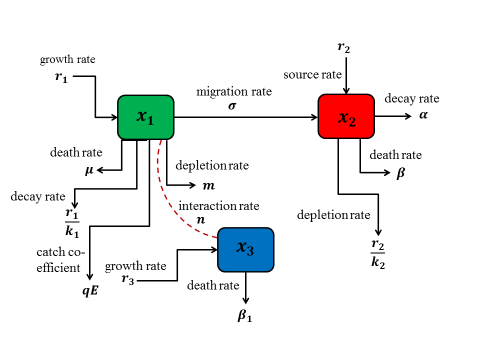
We consider a three compartmental model of fishery consisting of two zones: one is reserved where only prey species can reside while the other is unreserved zone where both prey and predator species can reside. Harvesting is permissible in unreserved zone but it is prohibited in reserved zone. The prey species can migrate from unreserved to reserved area while the vice versa is restricted. Keeping all these in view, the schematic diagram of the interaction among the fish species and predator in two zones has been shown in Figure 1.
Figure 1. Compartmental fishery of prey predator fishery in different zones
Taking the diagram represented in Figure 1 into consideration, the mathematical model of the prey predator fishery can be written as
$\frac{d{{x}_{1}}}{dt}={{r}_{1}}{{x}_{1}}\left( 1-\frac{{{x}_{1}}}{{{k}_{1}}} \right)-\left( \mu +\sigma +qE \right){{x}_{1}}-\frac{m{{x}_{1}}{{x}_{3}}}{a+{{x}_{1}}}$ (1)
$\frac{d{{x}_{2}}}{dt}={{r}_{2}}{{x}_{2}}\left( 1-\frac{{{x}_{2}}}{{{k}_{2}}} \right)-\beta {{x}_{2}}-\alpha {{x}_{2}}+\sigma {{x}_{1}}\text{ }$ (2)
$\frac{d{{x}_{3}}}{dt}={{r}_{3}}{{x}_{3}}\left( 1-\frac{{{x}_{3}}}{{{k}_{3}}} \right)+\frac{n{{x}_{1}}{{x}_{3}}}{a+{{x}_{1}}}-{{\beta }_{1}}{{x}_{3}}\text{ }$ (3)
$\text{with }{{x}_{1}}\left( 0 \right)\ge 0,\text{ }{{x}_{2}}\left( 0 \right)\ge 0\text{ and }{{x}_{3}}\left( 0 \right)\ge 0.$ (4)
Here, x1(t) denotes the biomass density of prey fish species (black tiger prawn) in unreserved zone, x2(t) represents the biomass density of same species in reserved zone and x3(t) denotes the biomass density of predator fish species in unreserved zone. In this model, it is considered that the predator consumes the prey population as an alternative food. Here, r1, r2 and r3 represents the intrinsic growth rate of the prey and predator species in both zone respectively. k1, k2 and k3 are the environment carrying capacity of prey and the predator species respectively. Therefore, $\frac{{{r}_{i}}x_{i}^{2}}{{{k}_{i}}}$ (i=1,2,3) is the amount by which the fish species decrease due to the interaction among themselves. Let E be the total effort applied for harvesting the prey population in the unreserved area and q is the catch ability coefficient, σ be the migration rate of the prey from unreserved to reserved area. We consider μ is the natural death rate of the species in the unreserved area. Therefore, (μ+σ+qE)x1 is the number of prey population that has been decreased from unreserved area due to fishing, migration and death rate. Let m be the depletion rate of prey species due to predation and n be the growth rate of the predator due to consumption. So, $\frac{m{{x}_{1}}{{x}_{3}}}{a+{{x}_{1}}}$ is the depleted number of prey due to the interaction with predator species. Here, a denotes the saturation constant. Let β be the death rate of prey in reserved area due to disease and a be the rate at which the prey population may be stolen due to insecurity. The term (α+β)x2 denotes the number by which the prey population decreases from the reserved area. In this prey predator system, we have considered Holling type II functional response to show the interaction between prey and predator species.
The model (1)-(3) had been analyzed in order to describe the dynamics of the fish species. For the analysis of the model the following studies were considered:
3.1 Boundedness of the model
To prove that the model system is biologically well posed the following Lemma was to be satisfied.
Lemma 1: The set
$\Omega =\left\{ \left( {{x}_{1}},{{x}_{2}},{{x}_{3}} \right):w\left( t \right)={{x}_{1}}\left( t \right)+{{x}_{2}}\left( t \right)+{{x}_{3}}\left( t \right),0<w\left( t \right)<\frac{\delta }{\eta } \right\}$
attracts all solutions initiating in the interior of the positive orthant, where η is a constant and
$\mu \text{=}\frac{{{k}_{1}}}{4{{r}_{1}}}{{({{r}_{1}}+\eta -\mu -qE)}^{2}}+\frac{{{k}_{2}}}{4{{r}_{2}}}{{({{r}_{2}}+\eta -\beta -\alpha )}^{2}}+\frac{{{k}_{3}}}{4{{r}_{3}}}{{({{r}_{3}}+\eta )}^{2}}$
Proof: Let, $w\left( t \right)={{x}_{1}}\left( t \right)+{{x}_{2}}\left( t \right)+{{x}_{3}}\left( t \right),\text{ }\eta >0$ be a constant. Then we can write,
$\begin{align} & \frac{dw}{dt}+\eta w=\left( {{r}_{1}}+\eta -\mu -qE \right){{x}_{1}}-\frac{{{r}_{1}}}{{{k}_{1}}}{{x}_{1}}^{2}+\left( {{r}_{2}}+\eta -\alpha -\beta \right){{x}_{2}}-\frac{{{r}_{2}}}{{{k}_{2}}}{{x}_{2}}^{2} \\ & -\left( m-n \right)\frac{{{x}_{1}}{{x}_{3}}}{a+{{x}_{1}}}+\left( {{r}_{3}}+\eta -{{\beta }_{1}} \right){{x}_{3}}-\frac{{{r}_{3}}}{{{k}_{3}}}{{x}_{3}}^{2} \\ \end{align}$
Since m is the depletion rate coefficient of prey due to its intake by the predator and n is the growth rate coefficient of predator due to its interaction with their prey, so it is assumed that m≥n. Now η is chosen such that 0<η<β1.
$\begin{align} & \frac{dw}{dt}+\eta w\le \frac{{{k}_{1}}}{4{{r}_{1}}}{{\left( {{r}_{1}}+\eta -\mu -qE \right)}^{2}}+\frac{{{k}_{2}}}{4{{r}_{2}}}{{\left( {{r}_{2}}+\eta -\alpha -\beta \right)}^{2}} \\ & +\frac{{{k}_{3}}}{4{{r}_{3}}}{{\left( {{r}_{3}}+\eta \right)}^{2}} \\\end{align}$
By using differential inequality, we get,
$0<w({{x}_{1}}(t),{{x}_{2}}(t),{{x}_{3}}(t))\le \frac{\delta }{\eta }(1-{{e}^{-\eta t}})+({{x}_{1}}(0),{{x}_{2}}(0),{{x}_{3}}(0)){{e}^{-\eta t}}$
Taking limit as t→∞, we get, 0<w(t)≤δ/η.
3.2 Positivity of the solution of the model
Lemma 2: For${{x}_{1}}\left( 0 \right)\ge 0,{{x}_{2}}\left( 0 \right)\ge 0,{{x}_{3}}\left( 0 \right)\ge 0$, the solutions ${{x}_{1}}\left( t \right),{{x}_{2}}\left( t \right),{{x}_{3}}\left( t \right)$ are all non-negative for all t≥0
Proof: For positivity, equation (2.1) can be written as, $\frac{d{{x}_{1}}}{dt}\ge -\left( \mu +\sigma +qE \right){{x}_{1}}$ $\Rightarrow \frac{d{{x}_{1}}}{{{x}_{1}}}\ge -kdt$ where,$k=\left( \mu +\sigma +qE \right)$ $\Rightarrow {{x}_{1}}\ge {{c}_{1}}{{e}^{-kt}}$, where c1 is an integrating constant. Applying the initial condition, at $t=0,{{x}_{1}}\left( 0 \right)\ge 0$, we get, ${{x}_{1}}\left( 0 \right)={{c}_{1}}$. Putting the value of c1 in the equation, we get, ${{x}_{1}}\left( t \right)\ge {{x}_{1}}\left( 0 \right){{e}^{-kt}}$. When $t\to \infty ,{{x}_{1}}\left( t \right)\ge 0$. Therefore x1(t) is positive for all t≥0. Again equation (2.2) can be written as $\frac{d{{x}_{2}}}{dt}\ge -\left( \alpha +\beta \right){{x}_{2}}$ $\Rightarrow \frac{d{{x}_{2}}}{{{x}_{2}}}\ge -Ldt$, where $L=\left( \alpha +\beta \right)$. Integrating we get, ${{x}_{2}}\left( t \right)\ge {{c}_{2}}{{e}^{-Lt}}$, where c2 is an integrating constant. Applying the initial condition, at $t=0,{{x}_{2}}\left( 0 \right)\ge 0$, we get, ${{x}_{2}}\left( 0 \right)={{c}_{2}}$. Putting the value of c2, we get, ${{x}_{2}}\left( t \right)\ge {{x}_{2}}\left( 0 \right){{e}^{-Lt}}$. When $t\to \infty ,\text{ }{{x}_{2}}\left( t \right)\ge 0$. Hence x2(t) is positive for all t≥0. To prove that x3(t) is positive, equation (2.3) is written as, $\frac{d{{x}_{3}}}{dt}\ge -{{\beta }_{1}}{{x}_{3}}$ $\Rightarrow \frac{d{{x}_{3}}}{{{x}_{3}}}\ge -{{\beta }_{1}}dt$. Integrating ${{x}_{3}}(t)\ge {{c}_{3}}{{e}^{-{{\beta }_{1}}t}}$, where c3 is an integrating constant. Now, at $t=0,{{x}_{3}}\left( 0 \right)\ge 0.$
So, ${{x}_{3}}\left( 0 \right)={{c}_{3}}.$
Putting the value of c3, we obtain, ${{x}_{3}}\left( t \right)\ge {{x}_{3}}\left( 0 \right){{e}^{-{{\beta }_{1}}t}}$. At $t\to \infty ,\text{ }{{x}_{3}}\left( t \right)\ge 0$. Therefore, x3(t) is positive for all t≥0. Hence this completes the proof.
3.3 Existence of equilibria
Let $\left( {{{\bar{x}}}_{1}},{{{\bar{x}}}_{2}},0 \right)$ be the positive solution of the equations (1) and (2)
${{\varphi }_{1}}{{x}_{1}}-\frac{{{r}_{1}}{{x}_{1}}^{2}}{{{k}_{1}}}=0$ (5)
$\frac{d{{x}_{2}}}{dt}={{\varphi }_{2}}{{x}_{2}}-\frac{{{r}_{2}}{{x}_{2}}^{2}}{{{k}_{2}}}+\sigma {{x}_{1}}\text{=0 }$ (6)
where, ${{\varphi }_{1}}={{r}_{1}}-\mu -\sigma -qE$and ${{\varphi }_{2}}={{r}_{2}}-\alpha -\beta $. From (5), we get, ${{x}_{1}}=0,{{\bar{x}}_{1}}=\frac{{{\varphi }_{1}}{{k}_{1}}}{{{r}_{1}}}$. Putting the value of ${{\bar{x}}_{1}}$in (6), we get,
${{\bar{x}}_{2}}=\frac{{{\varphi }_{2}}\pm \sqrt{\varphi _{2}^{2}+\frac{4\sigma {{r}_{2}}{{k}_{1}}{{\varphi }_{1}}}{{{r}_{1}}{{k}_{2}}}}}{\frac{2{{r}_{2}}}{{{k}_{2}}}}$
Again, let ($x_{1}^{*},x_{2}^{*},x_{3}^{*}$ ) be the positive solution of the equations
${{\varphi }_{1}}{{x}_{1}}-\frac{{{r}_{1}}{{x}_{1}}^{2}}{{{k}_{1}}}-\frac{m{{x}_{1}}{{x}_{3}}}{a+{{x}_{1}}}=0$ (7)
${{\varphi }_{2}}{{x}_{2}}-\frac{{{r}_{2}}{{x}_{2}}^{2}}{{{k}_{2}}}+\sigma {{x}_{1}}\text{=0 }$ (8)
${{\varphi }_{3}}{{x}_{3}}+\frac{n{{x}_{1}}{{x}_{3}}}{a+{{x}_{1}}}-\frac{{{r}_{3}}{{x}_{3}}^{2}}{{{k}_{3}}}=0$ (9)
where, ${{\varphi }_{3}}={{r}_{3}}-{{\beta }_{1}}$. Equation (9) yields
${{x}_{3}}=0,\text{ }a{{\varphi }_{3}}+{{\varphi }_{3}}{{x}_{1}}-\frac{a{{r}_{3}}{{x}_{3}}}{{{k}_{3}}}-\frac{{{r}_{3}}{{x}_{1}}{{x}_{3}}}{{{k}_{3}}}+n{{x}_{1}}=0$ $\Rightarrow {{x}_{1}}^{*}=\frac{a{{r}_{3}}{{x}_{3}}^{*}-a{{\varphi }_{3}}{{k}_{3}}}{{{\varphi }_{3}}{{k}_{3}}+n{{k}_{3}}-{{r}_{3}}{{x}_{3}}^{*}}$.
Using the value of ${{x}_{1}}^{*}$ in equation (8), we get
$\frac{{{r}_{2}}x_{2}^{{{*}^{2}}}}{{{k}_{2}}}-{{\varphi }_{2}}x_{2}^{*}-\sigma (\frac{a{{r}_{3}}x_{3}^{*}-a{{\varphi }_{3}}{{k}_{3}}}{{{\varphi }_{3}}{{k}_{3}}+n{{k}_{3}}-{{r}_{3}}x_{3}^{*}})=0$
This equation will have a positive solution if ${{\varphi }_{2}}\ge 0\Rightarrow {{r}_{2}}-\alpha -\beta \ge 0$. Finally from equation (3.3), we obtain
${{x}_{3}}^{*}=\frac{a+{{x}_{1}}^{*}}{m}\left( {{\varphi }_{1}}-\frac{{{r}_{1}}{{x}_{1}}^{*}}{{{k}_{1}}} \right)$
Hence the equilibrium points of the system are ${{P}_{1}}(0,0,0),{{P}_{2}}({{\bar{x}}_{1}},{{\bar{x}}_{2}},0)\text{ and }{{P}_{3}}\left( {{x}_{1}}^{*},{{x}_{2}}^{*},{{x}_{3}}^{*} \right)$.
3.3 Stability analysis at steady state
The Jacobean of the system is
$J\left( {{x}_{1}},{{x}_{2}},{{x}_{3}} \right)=\left( \begin{align} & {{\text{r}}_{1}}\text{-}\frac{2{{r}_{1}}{{x}_{1}}}{{{k}_{1}}}\text{-}\left( \mu +\sigma +qE \right)\text{-}\frac{am{{x}_{3}}}{{{\left( a+{{x}_{1}} \right)}^{2}}}\text{ 0 -}\frac{m{{x}_{1}}}{a+{{x}_{1}}} \\ & \text{ }\sigma \text{ }{{\text{r}}_{2}}\text{-}\frac{2{{r}_{2}}{{x}_{2}}}{{{k}_{2}}}\text{-}\beta -\alpha \text{ 0} \\ & \text{ }\frac{an{{x}_{3}}}{{{\left( a+{{x}_{1}} \right)}^{2}}}\text{ 0 }{{\text{r}}_{3}}-\frac{2{{r}_{3}}{{x}_{3}}}{{{k}_{3}}}\text{-}{{\beta }_{1}} \\ \end{align} \right)$ $\therefore \text{ }J\left( 0,0,0 \right)=\left( \begin{align} & {{\text{r}}_{1}}-\left( \mu +\sigma +qE \right)\text{ 0 0} \\ & \text{ }\sigma \text{ }{{\text{r}}_{2}}\text{-}\beta -\alpha \text{ 0} \\ & \text{ 0 0 }{{\text{r}}_{3}}-{{\beta }_{1}} \\\end{align} \right)$
Then the characteristics equation of the matrix with eigenvalue λ is
$\left| J-\lambda I \right|=\left| \begin{align} & {{\text{r}}_{1}}-\left( \mu +\sigma +qE \right)\text{-}\lambda \text{ 0 0} \\ & \text{ }\sigma \text{ }{{\text{r}}_{2}}\text{-}\beta -\alpha -\lambda \text{ 0} \\ & \text{ 0 0 }{{\text{r}}_{3}}-{{\beta }_{1}}-\lambda \\\end{align} \right|=0$
$\Rightarrow {{\text{r}}_{1}}-\left( \mu +\sigma +qE \right)\text{-}\lambda =0,\text{ }{{\text{r}}_{2}}\text{-}\beta -\alpha -\lambda =0\text{ or }{{\text{r}}_{3}}-{{\beta }_{1}}-\lambda =0$
$\Rightarrow {{\lambda }_{1}}={{\text{r}}_{1}}-\left( \mu +\sigma +qE \right),\text{ }{{\lambda }_{2}}={{\text{r}}_{2}}\text{-}\beta -\alpha \text{ and }{{\lambda }_{3}}={{\text{r}}_{3}}-{{\beta }_{1}}$
The eigenvalue λ of the matrix determines the stability of the states. Depending on λ, the stability conditions are: 1. if the eigenvalue λ>0, then the steady state is unstable, 2. if the eigenvalue λ<0, then the system is stable.
In the following lemma, we show that ${{P}_{3}}(x_{1}^{*},x_{2}^{*},x_{3}^{*})$ is locally asymptotically stable.
Lemma 3. The equilibrium point ${{P}_{3}}(x_{1}^{*},x_{2}^{*},x_{3}^{*})$ is always locally asymptotically stable.
Proof: Let, the three functions be $u=u\left( {{x}_{1}},{{x}_{2}},{{x}_{3}} \right),v=v\left( {{x}_{1}},{{x}_{2}},{{x}_{3}} \right)\text{ and }w=w\left( {{x}_{1}},{{x}_{2}},{{x}_{3}} \right)$ of the system (2.1)-(2.3). Then the Jacobean at ${{P}_{3}}(x_{1}^{*},x_{2}^{*},x_{3}^{*})$ is
${{J}_{3}}(x_{1}^{*},x_{2}^{*},x_{3}^{*})=\left( \begin{align} & {{\text{r}}_{1}}\text{-}\frac{2{{r}_{1}}{{x}_{1}}^{*}}{{{k}_{1}}}\text{-}\left( \mu +\sigma +qE \right)\text{-}\frac{am{{x}_{3}}^{*}}{{{\left( a+{{x}_{1}}^{*} \right)}^{2}}}\text{ 0 }\frac{m{{x}_{1}}^{*}}{a+{{x}_{1}}^{*}} \\ & \text{ }\sigma \text{ }{{\text{r}}_{2}}\text{-}\frac{2{{r}_{2}}{{x}_{2}}^{*}}{{{k}_{2}}}\text{-}\beta -\alpha \text{ 0} \\ & \text{ }\frac{an{{x}_{3}}^{*}}{{{\left( a+{{x}_{1}}^{*} \right)}^{2}}}\text{ 0 }{{\text{r}}_{3}}-\frac{2{{r}_{3}}{{x}_{3}}^{*}}{{{k}_{3}}}\text{-}{{\beta }_{1}} \\ \end{align} \right)$
Then the characteristics equation of the matrix with eigenvalue is λ.
|J-λI|=0
$\left| \begin{align} & {{\text{r}}_{1}}\text{-}\frac{2{{r}_{1}}{{x}_{1}}^{*}}{{{k}_{1}}}\text{-}\left( \mu +\sigma +qE \right)\text{-}\frac{am{{x}_{3}}^{*}}{{{\left( a+{{x}_{1}}^{*} \right)}^{2}}}\text{-}\lambda \text{ 0 -}\frac{m{{x}_{1}}^{*}}{a+{{x}_{1}}^{*}} \\ & \text{ }\sigma \text{ }{{\text{r}}_{2}}\text{-}\frac{2{{r}_{2}}{{x}_{2}}^{*}}{{{k}_{2}}}\text{-}\beta -\alpha -\lambda\text{ 0} \\ & \text{ }\frac{an{{x}_{3}}^{*}}{{{\left( a+{{x}_{1}}^{*} \right)}^{2}}}\text{ 0 }{{\text{r}}_{3}}-\frac{2{{r}_{3}}{{x}_{3}}^{*}}{{{k}_{3}}}\text{-}{{\beta }_{1}}-\lambda \\\end{align} \right|=0$
$\begin{align} & \Rightarrow \left( {{\text{r}}_{1}}\text{-}\frac{2{{r}_{1}}{{x}_{1}}^{*}}{{{k}_{1}}}\text{-}\left( \mu +\sigma +qE \right)\text{-}\frac{am{{x}_{3}}^{*}}{{{\left( a+{{x}_{1}}^{*} \right)}^{2}}}\text{-}\lambda \right)\left( {{\text{r}}_{2}}\text{-}\frac{2{{r}_{2}}{{x}_{2}}^{*}}{{{k}_{2}}}\text{-}\beta -\alpha -\lambda \right) \\ & \left( {{\text{r}}_{3}}-\frac{2{{r}_{3}}{{x}_{3}}^{*}}{{{k}_{3}}}\text{-}{{\beta }_{1}}-\lambda \right)+\left( \frac{m{{x}_{1}}^{*}}{a+{{x}_{1}}^{*}} \right)\left( \frac{an{{x}_{3}}^{*}}{{{\left( a+{{x}_{1}}^{*} \right)}^{2}}} \right)\left( {{\text{r}}_{2}}\text{-}\frac{2{{r}_{2}}{{x}_{2}}^{*}}{{{k}_{2}}}\text{-}\beta -\alpha -\lambda \right) \\\end{align}=0$$\Rightarrow \left( {{A}_{1}}\text{-}\lambda \right)\left( {{A}_{2}}-\lambda \right)\left( {{A}_{3}}-\lambda \right)+{{A}_{4}}\left( {{A}_{2}}-\lambda \right)=0$
$\Rightarrow {{\lambda }^{3}}+{{a}_{1}}{{\lambda }^{2}}+{{a}_{2}}\lambda +{{a}_{3}}=0$ (10)
where,
${{a}_{1}}=-\left( {{A}_{1}}+{{A}_{2}}-{{A}_{3}} \right),{{a}_{2}}=\left( {{A}_{1}}{{A}_{2}}+{{A}_{2}}{{A}_{3}}+{{A}_{3}}{{A}_{1}}+{{A}_{4}} \right),{{a}_{3}}=-\left( {{A}_{1}}{{A}_{2}}{{A}_{3}}+{{A}_{2}}{{A}_{4}} \right)$,
$\begin{align} & {{A}_{1}}={{\text{r}}_{1}}\text{-}\frac{2{{r}_{1}}{{x}_{1}}^{*}}{{{k}_{1}}}\text{-}\left( \mu +\sigma +qE \right)\text{-}\frac{am{{x}_{3}}^{*}}{{{\left( a+{{x}_{1}}^{*} \right)}^{2}}},\text{ }{{A}_{2}}={{\text{r}}_{2}}\text{-}\frac{2{{r}_{2}}{{x}_{2}}^{*}}{{{k}_{2}}}\text{-}\beta -\alpha ,\text{ } \\ & {{A}_{3}}={{\text{r}}_{3}}-\frac{2{{r}_{3}}{{x}_{3}}^{*}}{{{k}_{3}}}\text{-}{{\beta }_{1}},\text{ }{{A}_{4}}=\left( \frac{m{{x}_{1}}^{*}}{a+{{x}_{1}}^{*}} \right)\left( \frac{an{{x}_{3}}^{*}}{{{\left( a+{{x}_{1}}^{*} \right)}^{2}}} \right) \\\end{align}$
By Routh-Hurwitch criterion, all the eigenvalues of (3.7) have negative real roots if and only if a1>0, a3>0 and a1a2>a3.
Then the equilibrium point ${{P}_{3}}(x_{1}^{*},x_{2}^{*},x_{3}^{*})$ is locally asymptotically stable.
In this section, some numerical simulations of our proposed model were presented to investigate the dynamical behavior of the model. To do these simulations, MATLAB ode45 solver was used. The description and values of all parameters used in our proposed model are presented in Table 1.
Table 1. Description of parameters and their values
|
Symbols |
Description of parameters |
Values |
|
r1 r2 r3 $\sigma $ $\alpha$ $\beta$ ${{\beta }_{1}}$ $\mu$ m n a k1 k2 k3 |
intrinsic growth rate of black tiger prawn in unreserved area intrinsic growth rate of black tiger prawn in reserved area intrinsic growth rate of predator population in unreserved area migration rate decay rate due to being stolen (illegal pouching) death rate due to disease death rate of predator death rate of prey in unreserved area depletion rate of prey due to the predation growth rate of predator due to predation saturation constant carrying capacity of black tiger prawn in unreserved area carrying capacity of black tiger prawn in reserved area carrying capacity of predator population in unreserved area |
5 6 1.5 2.5 0.2 0.9 0.05 0.02 0.5 0.05 20 100 200 100 |
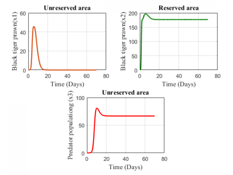
A time interval of 70 days was considered to show the dynamics. The figures displayed depict the densities of fish and predator population in reserved and unreserved area and shows where the population increases and decreases within 70 days. Figures 4.3-4.14 show the variation of black tiger prawn and predator population in two zones for changing values of different parameters.
The Figure 2 represents that fish population first increases, then decreases and finally grows at a constant rate in the unreserved area and the species in the reserved area first increases, then shows a slight decrease and finally grows at a constant rate. The predator population shows an increasing effect for the above values of the parameter.
Figure 3. Variation of population with time (70) days for
keeping all values sameFigure 3 illustrates that for the increasing values of depletion rate and growth rate due to predation, the black tiger prawn in the unreserved area increases in the first 9 days, then decreases for after 9 days and at last it extinct while in the reserved area it shows a slight changing effect. The figure also shows that the predator population increases for the parameter values.
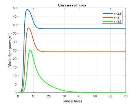
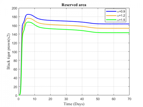
Figure 4. Variation of black tiger prawn inreserved area for different values of $\sigma$
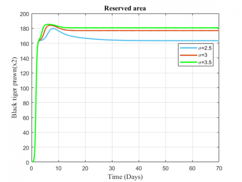
Figure 5. Variation of black tiger prawn in reserved area for different values of $\sigma$
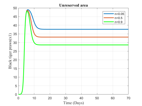
Figure 6. Variation of black tiger prawn in unreserved area for different values of n
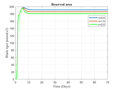
Figure 7. Variation of black tiger prawn in reserved area for different values of n
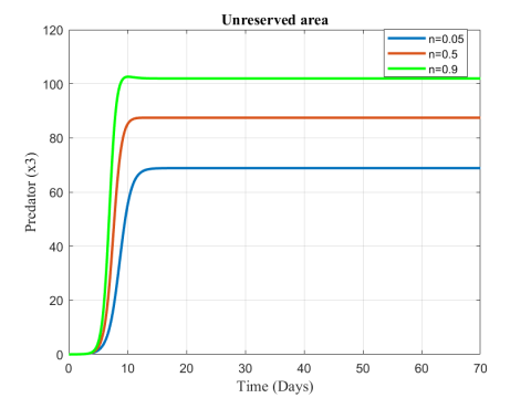
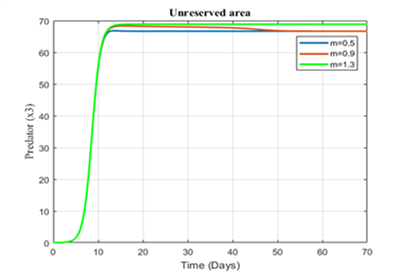
Figure 8. Variation of predator population in unreserved area for different values of n
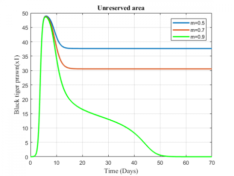
Figure 9. Variation of black tiger prawn for different values of m
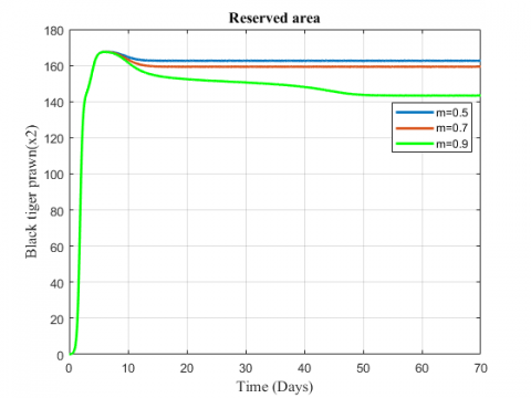
Figure 10. Variation of black tiger prawn in reserved area for different values of m
Figure 11. Variation of predator in the unreserved area for different values of m
The change in the biomass density of black tiger prawn in the two zones for increasing values of $\sigma$ has been represented in Figures 4 and 5. The fish population in the unreserved area decreases for the increasing value of migration rate while population in reserved area shows an increasing effect.
Figures 6-8 show the variation of fish and predator population for different values of consumption rate due to predation. It is seen from the Figures that black tiger prawn in both zones decreases and predator population increases due to the increasing values of n .
The variation of fish and predator population for different values of depletion rate due to predation is represented in Figures 9-11. It is seen from the figures that black tiger prawn in both zones decreases and predator population increases due to the increasing values of m . The fish population in unreserved area extinct after 50 days as depletion rate increases.
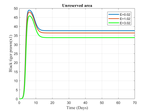
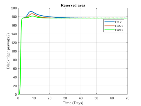
In Figures 12 and 13, we observe that fish population decreases from the unreserved area while the population increases in reserved area due to the increasing values of fishing or harvesting rate.
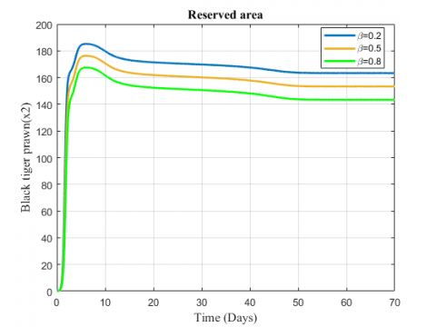
Figures 14 and 15 indicate the variation of black tiger prawn in reserved area for the changing values of the rate at which the species are stolen and death rate. Both the figures show a decreasing effect for the increasing values of $α$ and $β$ .
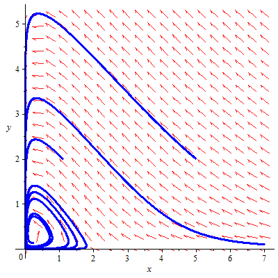
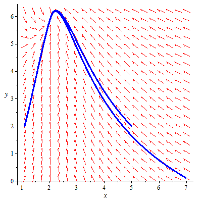
Some arbitrary data are assumed for describing the phase diagram of the system. Using the Maple2018 software, we have analyzed the stability analysis of the fishery model. The phase diagram of the model in presence and absence of predator in both reserved and unreserved area has been analyzed for the system. Figures 16 and 17 describe the phase diagram of the system.
Figure 12. Variation of black tiger prawn in unreserved area for different values of E
Figure 13. Variation of black tiger prawn in reserved area for different values of E
Figure 14. Variation of black tiger prawn in the reserved area for different values of $α$
Figure 15. Variation of black tiger prawn in reserved area for different values of $\beta$
Figure 16. Phase space diagram of the system in the presence of predator in the unreserved area with the parameter values
${{r}_{1}}=1,\text{ }{{k}_{1}}=7,\text{ }m=6,\text{ }n=6,\text{ }a=7,$
$\text{ }{{k}_{3}}=9,\text{ }{{r}_{3}}=0.2,\text{ }\beta =0.4,\text{ }\mu =0.2,\text{ }\sigma =0.3,\text{ }qE=0.2$
Figure 17. Phase space diagram of the system in the absence of predator in the unreserved and reserved area with the parameter values
${{r}_{1}}=1,\text{ }{{k}_{1}}=7,\text{ }{{k}_{2}}=9,\text{ }{{r}_{2}}=0.5,\text{ }\mu =0.2,$
$\sigma =0.4,\text{ }qE=0.2,\beta =0.2,\alpha =0.1$
Considering two ecosystems, a mathematical model of fishery has been formulated in this paper. We have analyzed the behavior of the model, focusing on the parameters that are mainly responsible for the production and reduction of black tiger prawn. The numerical results reveal that the high mortality rate, fishing rate and predation rate of black tiger prawn in the unreserved area have a decreasing effect on the species in the reserved area. It also shows that the number of black tiger prawn increases in the reserved area due to the high migration from the unreserved area. When predation increases, the number of black tiger prawn in both reserved and unreserved area reduces by a significant amount. It is also evident from the simulations that the production of black tiger prawn in the reserved area decreases due to death from different diseases and for being stolen in absence of security. The main conclusion based on the result is that it is possible to maximize the production of black tiger prawn by proper management and thus it can play a significant role in the economy of a country.
The authors would like to thank the reviewers for the careful reading of this manuscript and their fruitful comments and suggestions for further modifications of this manuscript. Khatun greatly acknowledged the partial financial support during her Masters program provided by the National Science and Technology (NST) fellowship with the ref. no.39.00.0000.012.002.03.18, under Ministry of Science and Technology, Government of the People’s Republic of Bangladesh.
[1] Biswas MHA, Hossain MR, Mondal MK. (2017). Mathematical modeling applied to sustainable management of marine resources. Procedia Engineering 194: 337–344.https://doi.org/10.1016/j.proeng.2017.08.154
[2] Biswas MHA, Rahman T, Haque N. (2016). Modeling the potential impacts of global climate change in Bangladesh: an optimal control approach. Journal of Fundamental and Applied Science 8(1): 1-19. http://dx.doi.org/10.4314/jfas.v8i1.1
[3] Agarwal M, Pandey P. (2006). Combined harvesting of two competitive species having a resource dependent carrying capacity. Indian J. pure appl. Math. 37(2): 63-73.
[4] Chaudhury KS. (1986). A bioeconomic model of harvesting a multispecies fishery. Ecol. Model. 32(4): 267-279. https://doi.org/10.1016/0304-3800(86)90091-8
[5] Clark CW. (1979). Mathematical models in the economics of renewable resources. SIAM Rev. 21(1): 81-99. https://doi.org/10.1137/1021006
[6] Dubey B, Chandra P, Sinha P. (2003). A model for fishery resource with reserve area. Nonlinear Analysis: Real World Application 4(4): 625-637. https://doi.org/10.1016/S1468-1218(02)00082-2
[7] Mondal MK, Hanif M, Biswas MHA. (2017). A mathematical analysis for controlling the spread of Nipah virus infection. International Journal of Modeling and Simulation 37(3): 185-197. https://doi.org/10.1080/02286203.2017.1320820
[8] Dubey B, Chandra P, Sinha P. (2002). A resource dependent fishery model with optimal harvesting policy. J. Biol. Systems 10(1): 1-13. https://doi.org/10.1142/S0218339002000494
[9] Chaudhury KS. (1988). Dynamic optimization of combined harvesting of a two species fishery. Ecol. Model 41(1-2): 17-25. https://doi.org/10.1016/0304-3800(88)90041-5
[10] Kar TK. (2006). A model for fishery resource with reserve area and facing prey-predator interaction. Canadian Applied Mathematics Quarterly 14(4): 385-399.
[11] Roy B, Roy SK, Biswas MHA. (2017). Effects on prey-predator with different functional responses. Int. Journal of Biomathematics 10(8): 1750113-22. https://doi.org/10.1142/S1793524517501133
[12] Biswas MHA. (2014). On the evaluation of AIDS/HIV treatment: An optimal control approach. Current HIV Research 12(1): 1-12. https://doi.org/10.2174/1570162X1201140716094638
[13] Biswas MHA. (2013). Necessary conditions for optimal control problems with state constraints: Theory and applications. PhD Thesis, Department of Electrical and Computer Engineering, Faculty of Engineering, University of Porto, Portugal.
[14] Biswas MHA. (2012). AIDS epidemic worldwide and the millennium development strategies: A light for lives. HIV and AIDS Review 11(4): 87-94. https://doi.org/10.1016/j.hivar.2012.08.004
[15] Dym CL. (2004). Principles of Mathematical Modeling. Second Edition, Academia Press, New York.
[16] Louartassi Y, Alami JEl, Elalami N. (2017). Harvesting model for fishery resource with reserve area and modified effort function. Malaya J. Mat. 5(4): 660-666. https://doi.org/10.26637/MJM0504/0008
[17] Murray JD. (1993). Mathematical Biology, Second Edition, Springer-Verlag Berlin Heidelberg.
[18] Ross SL. (2004). Differential equation, Third Edition, Jhon Wiley & Sons, UK.
[19] Sarwardi S, Mandal PK, Ray S. (2013). Dynamic behavior of a two predator model with prey refuge. J. Biol. Phys. 39(4): 701-722. https://doi.org/10.1007/s10867-013-9327-7
[20] Zhang X, Chen L, Neuman AU. (2000). The stage structured predator-prey model and optimal harvesting policy. Math. Biosci. 168(2): 201-210. https://doi.org/10.1016/S0025-5564(00)00033-X
[21] Dubey B, Patra A. (2013). Optimal management of a renewable resource utilized by a population with taxation as a control variable. Nonlinear Analysis: Modeling and Control 18(1): 37-52.