OPEN ACCESS
The problems of contact are intrinsically non-linear owing to the fact that the surface of contact is unknown a priori. Usually, method contact and used within the framework of the method finite elements to deal with problems of contact.
The method of resolution of the contact has its own parameters of calculation. The latter can impact the results directly. This is why it is significant to use the method with precaution. To consolidate the results obtained, it is always necessary to carry out a study of sensitivity on these parameters and if need be, to use another method to make it possible to measure the results. In addition, each method has its advantages and its disadvantages. The method of penalization is easy to implement in a code of finite elements as Ansys but the principal disadvantage is the choice of the coefficients of penalization (stiffnesses of contact) which have a direct influence on the results. The method of the Lagrangian one which exists in the codes finite elements like Ansys, as for it, makes it possible to observe the condition of non penetration and to avoid the problems involved in the choice of the coefficients of penalization. On the other hand, it is more difficult to implement since it requires on the one hand the introduction of additional unknown factors (multipliers of Lagrange) and on the other hand it requires the definition of surfaces Masters and the nodes esclaves.
Mechanical Contact, Friction, Methods of contact, Finite elements.
The contact problem is non linear since the contact region is not known beforehand, and the boundary conditions may change during the analysis.A limited number of contact problems is sufficiently well behaved to have an analytical solution, such as the Hertz contact [1].
For this reason, contact problems are solved with numerical techniques in general.The most used technique to treat structural non linearities is the Finite Element method(FEM) [2, 3, 4, 5, 6] while the Boundary Element Method(BEM)has been recently employed in contact problems [7, 8, 9, 10], just to cite a few of the recent works.
The objective of this paper is to present a methodology to the estimation of contact stiffness, one of the main parameters of a contact problem in the commercial software ANSYS [2].
There are different methods for solving the contact. We present here the Lagrangian methods and the penalty. And, are applied on a case study industrial to remove the advantages and disadvantages of each methods.
We present in this section the main aspects of the contact formulation using the Augmented Lagrangian Method and Penalty Method how this methods is implemented in the ANSYS software.
2.1 Introduction to the static contact problem
The contact problem can be formulated as a constrained minimization problem, where the objective function to be minimized is the total potential energy Π( u) of the bodies in contact, and the constraints are given by non-penetration conditions between the bodies. Thus, the problem can be stated as
$\min \Pi(u)$
subject to $g_{j}(u) \leq 0$ $\mathrm{j}=1, \ldots, \mathrm{n}$ (1)
where u is the optimization variable(displacement vector) and gj(u) represents one of the n non-penetration constraints that can be defined as
The total potential energy Π( u) for the contact problem between two elastic bodies subjected to small deformations and small displacements(static problems)can be described as
$\Pi(u)=\Pi_{A}(u)+\Pi_{B}(u)=\frac{1}{2}\left\{\begin{array}{ll}u_{A} \\ u_{B}\end{array}\right\}^t\left[\begin{array}{cc}K_{A} & 0 \\ 0 & K_{B}\end{array}\right]\left\{\begin{array}{l}u_{A} \\ u_{B}\end{array}\right\}-\left\{\begin{array}{l}f_{A} \\ f_{B}\end{array}\right\}^{t}\left\{\begin{array}{l}u_{A} \\ u_{B}\end{array}\right\}$ (2)
where Ki is stiffness matrix, ui is the displacement field, fi is the external force, i represents an elastic body(i=A or i=B) and t denotes matrix transposition. For convenience, these variables are simplified to K, u and f from now.Thus, the total potential energy is given by
$\Pi(u)=\frac{1}{2} u^{t} K u-f^{t} u$ (3)
Several constrained minimization algorithms can be used to solve the problem of Eq. (1) such as the Penalty Method, the Lagrange Multipliers Method and the Augmented Lagrangian Method. The results presented in this paper are based on the Augmented Lagrangian Method according to the ANSYS implementation. This leads to the requirement of setting some contact parameters that are described in the next subsections together with a brief description of the Augmented Lagrangian and penalty method formulation.
3.1 Augmented Lagrangian method
The Augmented Lagrangian method is considered as a hybrid method of Lagrange Multipliers method and Penalty method.For more details about these algorithms, refer to [11] for instance.
The contact constraints are considered in this formulation using penalizing coefficients and Lagrange multipliers, penalizing the non-penetration restrictions violations in the same form of the Penalty method, and solving the constrained minimization problem through the solution of sequential un constrained minimization problems with the up dating of Lagrange multiplier sin the solution process. The Augmented Lagrangian function is given by
$L_{\text {aum}}=\Pi(u)+\lambda^{t} g(u)+\frac{1}{2} r[g(u)]^{2}$ (4)
where $[X]_{+}$ represents max(0; x), r is the penalizing coefficient and $g(u)=\left[g_{1}(u), g_{2}(u) \ldots \ldots g_{n}(u)\right]$ is the constraint vector and λ is the Lagrange multipliers vector.It is easy to verify that the Augmented Lagrangian function in corporate a penalization term and a Lagrange multiplier term. The gradient of the Augmented Lagrangian function is given by
$\nabla L_{aum}=\nabla \Pi(u)+\lambda^{t} \nabla g(u)+r[g(u)]+\nabla g(u)$ (5)
which allows to verify that at the optimum point u*, the penetration restriction fulfills g(u*)=0. In this case we have
$\nabla L_{aum}=\nabla \Pi\left(u^{*}\right)+\lambda^{t} \nabla g(u *)=0$ (6)
3.2 Penalty method
The penalty method is a classical and widespread method for the numerical treatment of constrained problems, in particular the unilateral contact problems arising in mechanics of deformable bodies which involve a nonlinear boundary condition written as an inequality (see, e.g., [12, 13, 14]). Nevertheless, and to the best of our knowledge, the convergence analysis of the method in the simplest case of linear elasto statics with or without finite element discretization has been object of few studies. We may nevertheless quote the earlier, and pioneering works of Kikuchi, Kim, Oden and Song [15, 16, 17] (see also [12]) and the more recent study dealing with the boundary element method [18].
The method of penalty is to introduce this requirement in the functional of the total energy in the following form
$\bar{\pi}\left(X_{t}\right)=\pi\left(X_{t}\right)+\frac{\chi}{2} \cdot x_{t}^{t} x_{t}$ (7)
Xt with the nodal displacement vector at time t, xt is the vector of nodal interstices at time t is the coefficient of penalization and functional of the total energy associated with the body in contact. in minimizing the functional (7), the discrete variational equation which is associated:
$\delta \pi\left(x_{t}\right)=\chi \cdot x_{t}^{t} \cdot x_{t}=0$ (8)
proposed to determine the function of parameters such as:
$\chi_{\bar{n}}=\chi_{\bar{t}}=\alpha \frac{A^{2} \cdot K}{V}$ (9)
With A the area of the surface of the contact element, V is the volume of this element, K buckling module and a scale factor to be addressed and taken generally equal to 0.1 [19].
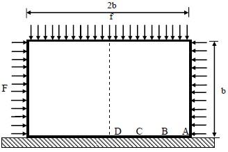
This example is often studied as a benchmark.It was proposed by Raous [20] and Feng [21]. This is a elastic block compressed copper alloy, in contact with a rigid foundation. The dimensions, loads and boundary conditions are shown on figure2. The different elements of the problem are summarized below:
Figure 1. Contact between an elastic block and a rigid foundation
For reasons of symmetry we took only the half of the block, with planar deformation.
Figure 2. Half of the elastic block in contact with the foundation
The mesh consists of 512 quadrilateral elements with 4 nodes. The contact surface is composed of 32 nodes.
(a) Method of Lagrange (b) Method of Penalty
Figure 3. Reactions of the contact surface
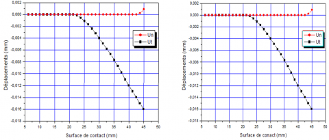
(a) Method of Lagrange (b) Method of Penalty
Figure 4. Displacements of the contact surface
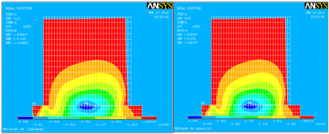
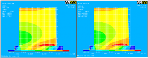
The elastic block in terms of distribution of the shear stress and distribution of Von Mises stresses as shown in the figure below:
(a) Method of Lagrange (b) Method of Penalty
Figure 5. distribution of the shear stress
(a) Method of Lagrange (b) Method of Penalty
Figure 6. Distribution of Von Mises stresses.
Figures (a) and (b) show that both methods give al most the same travel and the same contact reaction. We can see that the results depend on ANSYS penalty coefficient Kn can simultaneously have three different types of contact surfaces: Separation, Sliding, Adhesion A resilient block interface where contact occurs, for the same load factor, both methods give the same mechanical behavior. In effect, the two methods indicated the identified separation zones.
The results are in good agreement.
In this study, we presented the penalty method and Lagrangian, each contact resolution method has its own calculation parameters. This is why it is important to use these methods carefully to consolidate the results. Each method has its advantages and disadvantages. The penalty method is easy to implement in a finite element code ANSYS like but the main disadvantage is the choice of penalty coefficients (contact stiffness) that have a direct influence on the results.
The Lagrangian method that exists in finite element codes such as ANSYS, in turn, allows to observe the condition of non penetration and avoid problems in the choice of penalty coefficients. By cons, it is more difficult to implement because it requires both the introduction of additional unknowns (Lagrange multipliers).
[1] H. Hertz, “On the contact on elastic solids,” J.Math., vol. 92, pp. 156–171, 1881. http:// home.uni-leipzig.de/pwm/web /download/ Hertz 1881.pdf
[2] ANSYS, “ANSYS Contact Technology Guide” 2005. https://www.sharcnet.ca/Software/Ansys/16.2.3/en.../ctectoc.html
[3] F.J.Cavalieri, A.Cardona, “Anaugmented Lagrangian technique combined with a mortar algorithm for modelling mechanical contact problems,” Int. J. Numer. Methods Eng., vol. 93, no. 4, pp. 420–442, 2013. DOI: 10.1002/nme.4391.
[4] A.R. Mijar, J.S. Arora, “An augmented Lagrangian optimization method for contact analysis problems,” Struct. Multidiscip. Optim., vol. 28, pp. 99–112, 2004. DOI: 10.1007/s00158-004-0423-y.
[5] D. Peric, D.R.J. Owen, “Computational model for 3-D contact problems with friction based on the penalty method,” Int. J. Numer. Methods Eng., vol. 35, pp. 1289–1309, 1992. DOI: 10.1002/nme.1620350609.
[6] M.A. Puso, T.A. Laursen, “Amortar segment-to-segment contact method for large deformation solid mechanics,” Comput. Methods Appl. Mech. Eng., vol. 193, pp. 601–629, 2004. https://e-reports-ext.llnl.gov/pdf/302054.pdf
[7] I. Benedetti, M.H. Aliabadi, “A three-dimensional cohesive-friction algrain- boundary micro mechanical model for intergranular degradation and failure in polycrystalline materials,” Comput. Methods Appl. Mech. Eng., vol. 265, pp. 36–62, 2013. https://scholar.google.com/citations?view_op=view_citation&hl=it&user=YnGi0JEAAAAJ&citation_for_view=YnGi0JEAAAAJ:kNdYIx-mwKoC
[8] H. Gun, X.W. Gao, “Analysis of frictional contact problems for functionally graded materials using BEM,” Eng. Anal. Bound. Elem., vol. 38, pp. 1–7, 2014.
[9] L. Rodríguez-Tembleque, F.C. Buroni, R. Abascal, A. Sáez , “Analysis of FRP composites under frictional contact conditions,” Int. J. Solids Struct., vol. 50, no. 24, pp. 3947–3959, 2013. DOI: 10.1016/j.ijsolstr.2013.08.007.
[10] L. Rodríguez-Tembleque, A. Sáez, F.C. Buroni, “Numerical study of polymer composites in contact,” Comput. Model. Eng. Sci., vol. 96, no. 2, pp. 131–158, 2013. DOI: 10.3970/cmes.2013.096.131.
[11] D.G. Luenberger, “Linear and Nonlinear Programming,” 2nd edition, Addison-Wesley Publishing Company, Reading, MA, USA, 1989.
[12] N. Kikuchi, J.T. Oden, “Contact Problems in elasticity: A study of variational inequalities and finite element methods,” SIAM Stud. Appl. Math., vol. 8, Society for Industrial and Applied Mathematics (SIAM), Philadelphia, PA, 1988.
[13] T.A. Laursen, “Computational contact and impact mechanics,” Springer-Verlag, Berlin, 2002. http:// www.springer.com/la/book/9783540429067
[14] P. Wriggers, “Computational Contact Mechanics,” Wiley, 2002. http://eu.wiley.com/WileyCDA/WileyTitle/productCd-0471496804.html
[15] N. Kikuchi, Y.J. Song, “Penalty-finite-element approximation of a class of unilateral problems in linear elasticity,” Quart. Appl. Math., vol. 39, pp. 1–22, 1981.
[16] J. Oden, N. Kikuchi, “Finite element methods for constrained problems in elasticity,” Internat. J. Numer. Methods Engrg., vol. 18, pp. 701–725, 1982. DOI: 10.1002/nme.1620180507.
[17] J. Oden, S. Kim, “Interior penalty methods for finite element approximations of the Signorini problem in elastostatics,” Comput. Math. Appl., vol. 8, pp. 35–56, 1982. DOI: 10.1016/0898-1221(82)90038-4.
[18] M. Chernov, A. Maischak, E. Stephan, “A priori error estimates for hp penalty bem for contact problems in elasticity,” Comput. Methods Appl. Mech.Engrg., vol. 196, pp. 3871–3880, 2007. http:// fulltext.study/preview/pdf/499978.pdf
[19] Helen Walter, “Modélisation 3D par éléments finis du contact avec frottement et de l’endommagement du béton: application a l’étude de fixations ancrées dans une structure en béton,” thèse de doctorat, institut national des sciences appliquées de lyon, 1999. http://theses.insa-lyon.fr/publication/ 1999ISAL0078 these.pdf
[20] Z.Q. Feng, “2D or 3D frictional contact algorithms and applications in a large deformation,” context, Comm. Numer. Meths. Eng., no. 11, pp. 409-416, 1995. http://lmee.univ-evry.fr/~feng/CNME95.pdf.
[21] Z.Q. Feng, “Some text examples of 2D and 3D Contact problems involving Coulomb Friction and large slip,” Math. Comput. Modeling, vol. 28, no. 4-8, pp. 469-477, 1998. DOI: 10.1016/S0895-7177(98)00136-8.