Wadie Bendali* | Ikram Saber | Mohammed Boussetta | Bensalem Bourachdi | Youssef Mourad
© 2022 IIETA. This article is published by IIETA and is licensed under the CC BY 4.0 license (http://creativecommons.org/licenses/by/4.0/).
OPEN ACCESS
The roll of consumption energy forecasting is very important to make planning of time-horizon strategy, and to mitigate a great energy management. As a result, improving the sustainability of energy, and creating a clean environment. Aiming to develop the forecasting of consumption energy in different time horizons, this work gives the results of a new hybrid method, which combine deep echo state network (DeepESN), with Binary genetic algorithm (BGA). DeepESN is an extension of Echo state network (ESN), which integrates the strong nonlinear time series processing capability (of ESN) with the advanced learning characteristic of the deep learning models. BGA is another version of genetic algorithm optimization methods that can be applied to find the best values of architecture hyperparameters of deep learning models, basesd on binary decoding of his chromosoms. In this work, we compared the accuracy and performance of proposed model DeepESN-BGA with other deep learning methods. It is found that DeepESN-BGA have a fast processing compared with other models. In addition, it gives best results based on error metrics, compared with DeepESN without BGA, and other deep learning models, in different time horizon forecasting. Proposed model has been compared also with DeepESN-DE, DeepESN-GA, and DeepESN-PSO aiming to evaluate the performance of BGA in term of deep learning optimization. DeepESN-BGA gives statistically good result compared with other hybrid models.
DeepESN, BGA, consumption power, optimization, forecasting
Energy is part of everyday life. Its role is extremely crucial; it is the driving force behind economic activity and personal and social development. On the one hand, due to the growth of human society with the increase of energy efficiency and the use of developed artificial intelligence techniques, on the other hand, the growth of population and economy leads to high energy consumption, which produces a major challenge [1]. Today, the world is facing a major double challenge in the field of energy. The first challenge is the lack of safe and adequate energy sources and the second is the large-scale renewable energy grid-connected power generation may have adverse effects on power grids [2]. Energy sectors around the world are under huge pressure to assure a stable and reliable energy supply. Depending on the data of BP Statistical Review of World Energy, in 2018, global primary energy consumption knows the biggest growth since 2013 by 2.8% [3].
The global transition to a smart grid is justified by the need to satisfy the ever-increasing electricity consumption and to guarantee the sustainable and secure supply of the power system [4]. Smart Grid is based essentially on integration of renewable energy sources [5]. In addition, many countries have opted for a renewable energy development policy due to rising oil prices and global climate change [6]. In these cases, forecasting of consumption power and renewable energy power production becomes more critical than ever before, in managing smart grid systems, which satisfies future sustainable needs. Under these circumstances, there are many methods for power forecasting, it can be classified to four main approaches: Mathematical approaches, machine learning approaches, deep learning approaches and hybrid approaches [7]. Mathematical technique has been applied in the past to predict power time series [8]. This can be classified into two categories: persistence model and statistical method. Unfortunately, it usually produces forecasts with poor accuracy and does not work well with non-linear data as well [8]. Because of these limitations, machine learning introduces better accuracy and performance, such as the SVM (Support Vector Machine) [9], ANN (Artificial Neural Network) [10], ELM (Extreme Learning Machine) [11].
In recent years, The ANN methods are developed, under the name of deep learning [12], which are considered complex machine learning models with many layers, hyper-parameters and algorithms for making a high accuracy and reality. Generally, deep learning used for three problems, regression (prediction), classification, and clustering [13]. As a result, it has many models used depend a nature of problems. RNN (Recurrent neuron network) is a famous one for power forecasting as a time series data [14, 15], because of his ability to memorize information from the previous states [14]. Recently RNN has developed in many forms as LSTM (long short-term memory), GRU (Gate recurrent units), and ESN (Echo state network) form to deal with problems such as vanishing gradient, exploding gradient, longtime training, and optimizing the flexibility of data training [16-18]. Both the consumption and production power are generally non-linear, volatile and uncertain. In this field, the Echo state Network (ESN) is the best due to his ability of modeling such kind of time series data [18]. ESN's hidden layer is replaced by a dynamic reservoir composed of several weakly connected neurons, that should make information processing easier [18]. In addition, during the learning process, only the read weights are trained on the basis of linear regression (LR) algorithms [18]. As a result, ESN has a fast convergence speed and can attain the overall optimal solution. In recent years, the introduction of many layers frameworks in the RNN has attracted much interest [15]. Recently, the Echo state network has been developed to have many architectures with additional layers and hyper-parameters under the name of DeepESN (Deep Echo State Network) [19]. It plays a very powerful learning role and in solving difficult time-series problems [19]. However, this type of deep learning architecture is typically developed by experts through trial and error, which takes a long time to obtain precise results [19]. Graphics processing unit (GPU) performance has increased significantly in recent years, which has led to the widespread use of reinforcement learning and evolutionary algorithms to make it possible to automate the process of finding the best model structure [20, 21]. Therefore, the use of a hybrid model combined between DeepESN and some optimization model can avoid the trial and error procedure and eventually obtain a strong increase in model performance. There are several methods to optimize forecasting models, generally, they can be classified into two big categories: Statistical methods, and Natural-inspired algorithms.
Starting with statistical methods, this kind of optimization models have a large bound of utilization in the field of energy forecasting, it is used to optimize the fitness function or loss function by finding the best hyperparameter or parameter values of the prediction model. The following lines show some works that used optimization statistical methods. Grid search (GS) was applied in [22] by Raviv et al., it is one of the basic methods that depend on finding the best values of hyperparameters, based on his performance metrics GS shift the values into the optimal point that represent optimal solution. By the way, in one of our articles [23] we used GS to optimize a hybrid model that constitutes from GRU and PCA methods to predict Global horizontal irradiations, choosing learning rate, bash size, dropout as optimized hyperparameters and MSE as loss function, so that gives a great result in term of efficiency and performance. Especially for neuron network parameters, Gradient Descent (GD) considered a conventional optimization algorithm that used to find the best weight values by moving to a minimum local point of fitness function. It has been reported in the literature that GD outperforms GS in the area of finding the best neuron network (Weight) parameters. It can be found countless papers that use GD, among them [24] written by Amarasinghe et al. Some studies as [25] and [26] use cross validation, which is applied mainly in the preprocessing of the data for prediction models. Generally, this method is applied in parallel to hyperparameters optimization, by splitting the datasets into one for training the model and different set to test optimized hyperparameters that make, to achieve the best one on a dataset. This method has many types including: K-fold cross-validation, leave p out cross-validation, hold-cross validation [27]. The community of researchers in the filed developing optimization methods applied other form of statistical and probabilistic methods in their works, which are named the family of Bayesian optimization. It is based on probabilistic equation to achieve the best objective function. Among the works that use these methods we found in Refs. [28, 29]. In this term, these papers find that Bayesian methods outperforms GS and CV methods. Nevertheless has a limitation, represented in that the covariance function parameters the must be tuned, which make the competition more complex [30]. There are also others statistical optimization approaches that are used in filed of energy forecasting as Quasi Newton Method which used by conzaleg et al. to optimize the weight in ARMAX model for time series forecasting [31]. Dynamic Integrated Forecast System Dicast applied by Sulaiman et al. [32]. Levenberg Marquardt used in [33] to optimize Self-recurrent wavelet NN (SRWNN) for short term load forecasting. Excavated association rules used in [34] for RBFNN hyperparameters optimization. Non-homogeneous poison process (NHPP) used by Yue et al. [35] and Altering Direction of Multiplier method used by Yu et al. [36].
In the field of energy forecasting, the natural-inspired algorithms have a big attraction by researchers and developers, e.g. for achieving a good efficient energy management, the paper [37] targets energy generation forecasting from renewable sources by using ANN model optimized by differential evolution (DE), which can deal with multiple hyperparameters of forecasting model. DE can be considered as a technique for the global optimization of nonlinear and non-differentiable continuous space functions or objective function. In literature, genetic algorithm (GA) used in many works related to prediction models situation. E.g. in [38], which used it to optimize hyper-parameters and parameters of Deep learning model with stacked auto-encoders aiming to forecast wind power. Moreover, GA was used in one of our works [39], with other form which is Binary GA (BGA), this version shows great result in term of architecture hyperparameters (i.e. number of units and number of layers) optimization of deep learning models (i.e. Simple RNN, LSTM, GRU). GA can be found also in another form, which named micro genetic algorithms (MGA), among the papers that used this method, we found [40], so that it was applied as an optimizer of weight of relevant vector machines, to predict electricity price. One of the most famous optimization algorithms is told Particle swarm optimization (PSO) that is used to look for the maximum or minimum of a function defined on a multidimensional vector space, which represent hyperparameters bound values. Raza et al. in [41] used both the gradient learning techniques and PSO to optimize the parameters of neuron networks as Feed forward neuron network (FFNN), back propagation neuron network (BPNN) to predict electricity load demand and he found that the gradient learning has a poor convergence performance, leading to inefficient model training. On the other hand, PSO address the optimization with height performance leading to obtain the best forecasting model. There are also many other natural inspired algorithms as Cuckoo Search Algorithms (CSA) using by Xiao et al. to optimize the coefficient weight of NN models [42], Modified firefly algorithm (MFA) which was used in many works, among them [43], which hybridize SVR with MFA to achieve better short-term load forecasting. Quasi oppositional artificial Bee colony optimization (QOABCO), which has a great impact to the forecasting model for electricity price and load, in the published work of Shayeghi et al. [44]. Novel shark search algorithm (NSSA) which is can be found in work [45], that represent an improved Elman NN by using (NSSA) to predict short-term load electricity. The family of meta-heuristic algorithms also applied in some works, as can be found in paper of Artich of Chou and Ngo [46], which used a hybrid version of ARMA and SVR model tuned using one of meta-heuristic methods. This family of methods can be seen also in [47], so that the authors here proposed an LSTM model aiming to forecast electricity price and demand, some hyperparameters of this model optimized using jaya optimization algorithm which is considered as one of the meta heuristic optimization family. Final natural inspired algorithm optimization method in our review is the Improved Environment Adaption Algorithm, which is applied by Singh et al. in his work [48], his application targets to tune the weights and the hyperparameters of ANN model, as a result giving to the model more precision and capability to overcome the over and under fitting issues. All of these methods can give relatively a pretty good result, by achieving the optimal values of certain parameters and hyperparmeters of Deep learning model. However, in the field of deep learning architecture optimization PSO, GA and DE are the most used. To summarize this related works, it is found that the PSO is the best one in term of accuracy compared with others but is suffering from low speed of computing. In addition, it is found that the GA achieves good fitness function value compared with DE. The BGA has significant optimization in this field and better in term of computing processing speed than simple GA.
In general, the hyperparameters can be divided into two categories training hyperparameters and architecture hyperparmeters [49]. The training hyperparameters are the variables which deal with how deep learning is trained (e.g. learning rate and bash size in RNN) or (e.g. Leaking rate and spectral radius in ESN). While the architecture hyperparmeters indicate the structure of network of deep learning. The BGA will be used in this work to select the best architecture of DeepESN by finding the adequate number of deep ESN units (neurons) and hidden layers, as result improving performance of DeepESN. In this study, a presentation of theoretical basis of ESN and DeepESN and there Architectural and learning hyperparameters will be presented, including different advantage of DeepESN compared with ESN in term of minimizing forecasting error and their ability to deal with long time series data as consumption power. This work also will show the capability of BGA to find best values of architectures hyperparameters. So that will be compared with other optimization algorithm as simple GA, PSO and DE. In addition, this paper gives a comparison of different hybrid deep learning models i.e. RNN-BGA, LSTM-BGA, GRU-BGA, ESN-BGA with DeepESN-BGA. The comparison of results will be based on MSE, RMSE and MAE as evaluation metrics to get the best model in term of accuracy, and it will base on computation time to compare the processing duration of different models.
In general, the motivations of this work are based in first on the optimisation of the architectural part of the DeepESN using binary genetic algorithms that can improve the prediction of the energy consumption by the deep learning mode. Testing the proposed model in the prediction of different cases of short-term time horizons. Achieving the best time computation with high accuracy and performance in different short horizons. Finally, finding the best way to deal with architectural hyperparameters of DeepESN, by testing different optimization models. The contribution of this study can be identified as follows:
• To the best of our knowledge, there is no work has optimized the architected hyperparameters of DeepESN by using our proposed model can improve the prediction operation of deep learning.
• The prediction in this work has been used for different time horizon (1 min, 5min, 10 min, 20 min) aiming to evaluate the model in different case of short-term prediction.
• A comparison between different deep learning models and DeepESN-BGA, in term of accuracy and time computation, deepESN has been shown great outperformance in this field.
• A comparison between hybrid DeepESN-BGA and other hybrid models i.e. DeepESN-GA, DeepESN-PSO, DeepESN-DE. This comparison is the first one for consumption power forecasting. BGA has been given optimal values of architecture hyperparameters (i.e. number of units of each layer, number of layers).
This paper is organized as follows: Section 2 general description of the data used for forecasting. Sections 3 for descriptions of GA and BGA and their proprieties. Sections 4 describe the basic ESN. Section 5 for proposed Deep ESN and their advantage respectively. Section 6 introduces the experimental models used and his application. Section 7 shows the representation of the results and the discussions. Finally, Section 8 for conclusions and summarizes the directions for future research.
Generally, there are four kinds of time horizon prediction, very short term, short term, medium term, and long time. Each of time horizon types has specific applications in smart grid. Very short term forecasting gives the prediction from 1 second to 30 minutes time range, it applied for power smoothers and the stability and regulation of grid systems. Short term forecasting has a time step of 1 h to 1 days, it is used for economic dispatch and unit commitment. Medium term concentrates on range of some weeks, this forecasting used for maintenance scheduling. Finally, long term forecasting uses the range of months or years, it is applied for systems planning [50].
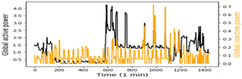
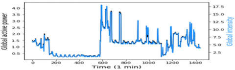
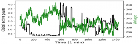
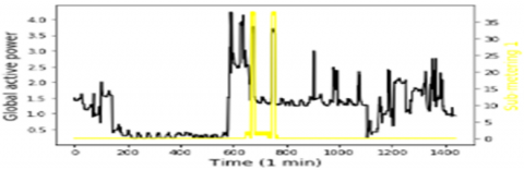
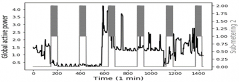
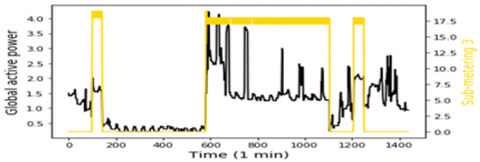
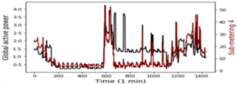
In this study, the data represents 1 min time step of multivariate data of active power consumption, this data are taken from a Households in Sceaux (7km of Paris, France) during 1 years. Which have 7 variables represent: Global active household power consumption (KW), the overall reactive power required by the household (KW), Means voltage (volts), Average current intensity (amps), Ea1, which is sub-measure of active energy for the kitchen (Wh), Ea2, which is Sub-measure of active energy for laundry (Wh), and Ea3, which is Sub-measure of active energy for climate control systems (Wh), all of this data represented in Figure 1. To obtain greater precision, the rest of active energy sub-measure Ea4, is included by using this equation.
$E a 4=(P a \times 1000 / 60)-(E a 1+E a 2+E a 3)$ (1)
Figure 1. Model input variables according to the global active power
3.1 Genetic algorithm
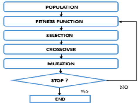
Nature has always been a great source of inspiration for all humankind. Genetic Algorithms (GA) are search algorithms based on the concepts of natural selection and genetics. GAs are a subset of a much larger branch of computing known as evolutionary computing. It is frequently used to solve optimization problems in research, specifically, in the task of parameters of machine learning and deep learning [51]. The GA process is divided into two parts:
• Identify the appropriate chromosomal encoding to be used as solutions or parameters to be tested.
• Determine the fitness function to be used to test the solutions obtained from the GA to determine if they are suitable to be used as next-generation solutions.
Genetic algorithms are carried out in different steps as shown in Figure 2 above. Firstly, it is important to initialize a population, which is a group of individuals who can solve the problem in question. An individual is characterized by a set of factors called genes and when these genes are linked together, they are called a chromosome and a group of chromosomes makes a population. After selection of the population, test the solutions got from GA whether it is appropriate to be used as a next generation solution or not by using fitness functions. In this study, Fitness Function is Mean Square Error (MSE).
The operation of mating the individuals makes a new solution from the old solutions, this operation named crossover, allowing the algorithms to have many solutions and to select the best of them. After this, mutation step, that gives to the solutions more variety, which can support the algorithms to be unpredictable and to be not blocked in an unending loop of selections or crossovers.
3.2 Binary genetic algorithm
Binary GA, is another version of GA, this version steal has the same algorithm method. The difference here in representation of individuals which are the solution of fitness function, so that it be initialized as binary number, to present a binary chromosomes of gens of 1 or 0, then BGA try to assemble these chromosomes to create a population of binary number. The fitness function is represented in function of chromosome. After selection of the population, test the solutions got from BGA whether it is appropriate to be used as a next generation solution or not by using fitness functions. The description of each step of the mechanism of BGA is presented as follow:
Figure 2. Flowchart of genetic algorithm
Firstly, it is important to define the fitness function which is minimized, the variables which represent in this work the architecture hyperparameters of the deep learning model, and all parameters related with BGA as number of bites per gen, population size, mutation rate, selection process, mating process, and convergence condition. Secondly, it must initialize population, according to the number of hyperparameters and the population size. Thirdly, the population, including the chromosome is decoded to produce a solution space of variables. Then, the fitness function of each chromosome is calculated and listed, aiming to minimize them. Additionally, the operation of natural selection is operated in the process, the BGA here create what is named offspring in each generation by making the selection of linked chromosomes, this operation based on selecting a set of fittest chromosomes from which the parent will be chosen, and all relative chromosomes are thrown and be substituted by produced offspring. Once the natural selection is finished, the mating step start. Generally, three approaches can be used to perform the mating: single point crossover, double point crossover and uniform crossover. In the first one, a random selecting of a crossover point between the first and last bit of the chromosomes by swapping the bites. In the second one, here the exchange of the chromosomes bites is existing between two crossover points. In the third one, the gens here are chosen arbitrary, based on one of the relative genes of the parent chromosomes. After the production of offspring, the mutation happens, that enable the BGA to give populations new information, in the case of less efficiency of population in term of cost, this population will be rejected during the next iteration. In this term, the mutation rate indicates the number of bits is mutated in the population. Finally, the Algorithm verifies whether all the given convergence condition is met. If they are met, the operation stops by achieving the most likely variables that can minimize the fitness function. If it is not, the iteration of several generations is activated by an algorithm, which repeats all of his process, including decoding, cost computation, mating and mutation.
Figure 3. Simple ESN architecture
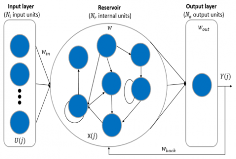
ESN represents one model from models of reservoir computing methods [52], with the strong simplification of his architecture as shown in Figure 3, it has a reservoir instead of hidden layer that make him offers a wide range of dynamic features. Among deference characteristics, it has capability to deal with nonlinear time series data very simply tanks of fully connected recurrent or simple units in his reservoir. These units are interlinked to achieve a high treatment efficiency and, accordingly, obtain good forecasts [19]. Typically, there are three kinds of neuron in ESN distributed such as this: $\frac{\mathrm{T}}{10}$ neurons of input layer that represent the variable input, $N_r$ neurons in reservoir layer shall be responsible for setting up inside information, and $N_o$ neurons in output layer which has forecasting data. Considering In time step j, the Eq. (2), (3) and (4) are respectively the input, hidden and output array of ESN represented as follows:
$U(j)=\left[U_1(j), U_2(j), U_3(j), \cdots, U_k(j)\right]^T$ (2)
$X(j)=\left[X_1(j), X_2(j), X_2(j), \cdots, X_n(j)\right]^T$ (3)
$Y(j)=\left[Y_1(j), Y_2(j), Y_2(j), \cdots, Y_o(j)\right]^T$ (4)
In ESN the reservoir and output states are adjusted under treatment by using Eqs. (5) and (6). As shown Figure 3, ESN architecture has four weight matrices, represents $w_{i n}$, that link the input and reservoir neurons, w for weighting the connection between reservoir units, $w_{b a c k}$ is a weight between output and reservoir, and $w_{\text {out }}$ in order to weight the connection of the reservoir units and output units.
$X(j+1)=F\left(w_{i n} U(j+1)+w X(j)+w_{\text {back }} Y(j)\right)$ (5)
$Y(j+1)=G\left(w_{\text {out }} X(j+1)\right)$ (6)
With F and G are the activation functions of the output and reservoir layers respectively. Depending on the characteristics of the data, these functions may be linear or non-linear. The choose of $w_{\text {in }}, w$ and $w_ {back}$ is random in the beginning, then remain the same [53, 54].
Generally, the principal hyperparmeters in ESN, are the spectral radius ρ, the LR algorithms, the connectivity rate, and the reservoir scale N. The connectivity rate α, which is showing the links of neurons inside the reservoirs. α can deal with sparsely or densely connecting of weights, as a result obtain a good reservoir reliability. In general, with reference to review of experience, α is chosen between 1%-5% [55]. The reservoir scale N, is a significant hyperparameter related to the total number of internal weights in the reservoir ($\mathrm{N}^2$). In general, N is linked to the level of complexity of the task and the sample size of the training. Same studies illustrate that the best values that can be chosen are between $\left[\frac{\mathrm{T}}{10}, \frac{\mathrm{T}}{2}\right]$, with T is the training samples size [55].
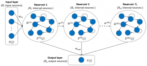
5.1 Architecture and algorithm of DeepESN
Figure 4. DeepESN architecture
DeepESN model is a new extended model of ESN, the most important character of DeepESN is the stacked hierarchy of reservoirs it could be has many reservoir layers as shown in Figure 4. The input of the first reservoir layer in each step j is equal to the outside input directly, while the previous layer output fed another reservoir layer. In order to make it more convenient, reservoir layers have identical number of neurons $N_r$. Moreover, $N_l$ indicate the total number of reservoir layers, and the $X^{\left[N_l\right]}(j)$ gives the states of the reservoir layer at time j, the reservoir states of the first layer and those layers at levels higher than 1 are updated with Eq. (7) and (8) respectively:
$X_{(j)}^{[1]}=F\left(w_{i n} \times U(j)+\widetilde{w}^{(1)} \times X^{[1]}(j-1)\right)$ (7)
$X_{(j)}^{[l]}=F\left(w^{(l)} \times X^{[l-1]}(j)+\widetilde{w}^{(l)} \times X^{[l]}(j-1)\right)$ (8)
$F=\left[F^{(1)}, F^{(2)} \ldots F^{\left(N_l\right)}\right]$ (9)
$F^{(l)}\left(l=1,2,3 \ldots, N_l\right)$ (10)
With $l=1,2,3 \ldots . N_l$, illustrate the evolution of reservoir states at layer l, assuming that F represents the function of activation for reservoir states in each layer (Eq. 9 and 10). DeepESN have weights metric as ESN model, in addition to $w^{(l)}$ matrix, which describe the relation between $N_l \times N_l$ represent the internal recurrent weights for layer l, and $\widetilde{w}^{(l)}$ the inter-layer connection weights from layer 1 to layer $N_l$, accordingly.
In ESN, each of the $w_{i n}$ and $w_{b a c k}$ is created at random according to a uniform distribution from the range [0, 1] and maintained throughout all phases of training, the same things for $w_{i n}$ and $w^{(l)}$ of DeepESN model. The w of ESN, and $\widetilde{w}^{(l)}$ of DeepESN are a scattered matrix initiated randomly, and they are scaled by using the relation as $\frac{\rho \times w}{\left|\gamma_{\max} \quad \right|}$ or $\frac{\rho^{(l)} \times \widetilde{w}^{(l)}}{\left|\gamma^{(l)}{ }_{\max } \quad \right|}$. With $\left|\gamma_{\max }\right|$ or $\left|\gamma^{(l)} \max\right|$ represent the spectral radius which is means the highest absolute intrinsic value of w, and ρ or $\rho^{(l)}$ is a hyperparametres of setting the spectral radius [56], with $l=1,2,3 \ldots ., N_l$. In order to enable the current internal states of the reservoir are simply associated with the input history over a few iterations, the spectral radius ρ has to be less than 1 [19, 55]. Within the learning procedure, only the $w_{\text {out }}$ has to be trained based on the LR algorithms, which allows for highly successful learning [56].
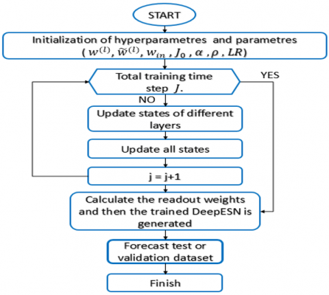
Figure 5. Flowchart of DeepESN method
As ESN model hyperparameters, the DeepESN has LR, connectivity rate α, spectral radius ρ, and instead of N, it has the reservoir scale $N_r$ in each reservoir. In addition, of these hyperparametres, the number of stacked reservoir layers $N_l$ is very important in DeepESN. For the calculation of output, Figure 3 illustrates how the state-output connected. The global stat is showed in Eq. (11), then it updates in Eq. (13). The relation between reservoirs and output layer are weighted by using $w_{\text {out }}$ of $N_o *\left(N_r * N_l\right)$. By using this connection state-output method, the playback component can attribute various weights to the dynamics supplied by each layer [57]. The output function is applied for collecting the complete state I of $\left(J-J_0+1\right) \times\left(N_r * N_l\right)$ and the target vector T of $\left(J-J_0+1\right) * N_o$, with the $J_0$ is the washout time step, based on condition of $J_0 \leq J$, after this compute the weights of the output based on this Eq. (12). Figure 5, represent the different steps of deepESN methods functionality.
$X(j)=\left[X_{(j)}^{(1)}, X_{(j)}^{(2)}, \ldots, X_{(j)}^{\left(N_l\right)}\right]$ (11)
$w_{\text {out }}=\left(I^{-1} * T\right)^t$ (12)
$Y(j)=w_{\text {out }} * X(j)$ (13)
5.2 Advantages of DeepESN
DeepESN have three advantages in comparison with simple ESN, among them:
This work aims to apply the advantage of DeepESN to deal with energy consumption prediction problems.
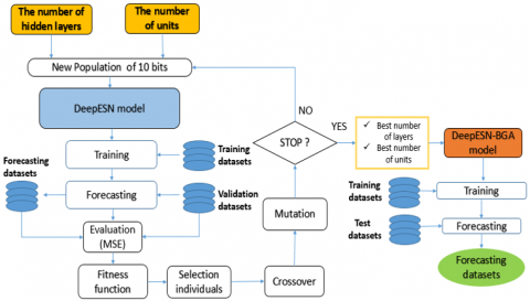
Figure 6. Flowchart of proposed model
In this study, the model of DeepESN has been developed using the Python framework created by C. Gallicchio [61] in 2018, named DeepESN framework. For using the BGA, this work based on Distributed Evolutionary Python (DEAP) library [63]. For the comparative prediction models, Keras has been used as a deep learning framework. The framework, which is used for other comparative optimization methods is mealy, it has many natural-inspired algorithms that can be applied to Deep learning models. All of these frameworks support the CPU and GPU hardware. It is found that the implementation of the proposed model is not expensive, and the requirements can be met with similar or more powerful hardware. The data in this study are normalized between 0 and 1, then they splatted into 60% for training, 20% for validation and 20% for testing.
Table 1. The hyperparameters values of prediction models
|
|
MLP |
RNN |
LSTM |
GRU |
ESN |
DeepESN |
DeepESN-PSO |
DeepESN-DE |
DeepESN-GA |
DeepESN-BGA |
|
Ni |
8 |
8 |
8 |
8 |
8 |
8 |
8 |
8 |
8 |
8 |
|
Nr |
20 |
18 |
17 |
17 |
20 |
20 |
[10,60] |
[10,60] |
[10,60] |
[10,60] |
|
Nl |
3 |
2 |
2 |
2 |
1 |
3 |
[2,10] |
[2,10] |
[2,10] |
[2,10] |
|
LR |
0.001 |
0.01 |
0.01 |
0.01 |
- |
- |
- |
- |
- |
- |
|
BS |
128 |
128 |
128 |
128 |
- |
- |
- |
- |
- |
- |
|
α |
- |
- |
- |
- |
0.05 |
0.03 |
0.03 |
0.03 |
0.03 |
0.03 |
|
ρ |
- |
- |
- |
- |
0.98 |
0.97 |
0.97 |
0.97 |
0.97 |
0.97 |
|
F |
Tanh |
Tanh |
Tanh |
Tanh |
Tanh |
Tanh |
Tanh |
Tanh |
Tanh |
Tanh |
|
G |
Relu |
Relu |
Relu |
Relu |
Relu |
Relu |
Relu |
Relu |
Relu |
Relu |
|
Epoches |
40 |
30 |
30 |
30 |
- |
- |
- |
- |
- |
- |
|
Dropout |
0.1 |
0.1 |
0.1 |
0.1 |
- |
- |
- |
- |
- |
- |
To obtain the adequate number of units and the number of layers (Figure 6). Firstly, the solutions of BGA initialized randomly, by decoding them from a binary array into decimal form. In order to optimize DeepESN, first the genetic algorithm will randomly initialize the values of a 10-bit binary array by using random Bernoulli distribution, corresponding to 4 bits for the number of layers and 6 bits for the number of units. Based on these values, the DeepESN trained given the Fitness function of the solutions in a current generation, in this phase, validation datasets used as input to forecast the active power of households. Then, the random Bernoulli distribution is equally applied for the random initialization of crossover, mutation and selection. In the end, the model that generates the minimum value of the fitness function, i.e. the one that provides the best numbers of layers and units, will be applied in the training and testing process, given the forecasting values. The values of optimization hyperparameters for DeepESN and ESN are selected by using the Trial and error method, including Spectral radius, and connectivity rate α. The activation function of the model is Tanh as hidden layers function, and Relu in output, all these parameters illustrate Table 1. Proposed model has been compared also with DeepESN-PSO, DeepESN-DE, DeepESN-GA, to evaluate the ability of BGA in term of optimizing architecture hyperparameters. The parameters of BGA and GA, which are chosen in this work, 3 for Generation number (GN), 10 for Genes size (Gs), and 4 as a populations size (PS). PSO tuned by using PS, local coefficient (LC), global coefficient (GC), weight minimum of bird (WBmin) and maximum of bird (WBmax). DE parameterized by using weighting factor (WF) and crossover rate (CR) in addition to PS. All parameter values of optimization methods (BGA, GA, DE, PSO) parameters are illustrate in Table 2. DeepESN-BGA also has been compared with other deep learning model, which are RNN, LSTM, GRU, MLP, ESN, and DeepESN without BGA, aiming to approve the efficiency and the performance of proposed model. The hyperparameters (bash size (BS), learning rate (LR)) of comparative models are selected by trial and error methods, the values of these hyperparmeters in addition of activation functions are illustrate also in Table 1. To evaluate the accuracy of the proposed model, it is important to use metric errors, in this work, root mean square error (RMSE), mean square error (MSE), and mean absolute error (MAE). The formulas of these metrics are shown in Eq. (14), (15), and (16)
$R M S E=\sqrt{\frac{1}{m} \sum_{i=1}^N\left(Y_{\text {forecast }}(t)-Y_{\text {true }}(t)\right)^2}$ (14)
$M A E=\frac{1}{m} \sum_{i=1}^N\left|Y_{\text {forecast }}(t)-Y_{\text {true }}(t)\right|$ (15)
$M S E=\frac{1}{m} \sum_{i=1}^N\left(Y_{\text {forecast }}(t)-Y_{\text {true }}(t)\right)^2$ (16)
With m is the number of samples, $Y_{\text {forecast }}(t)$ is the output of the prediction models at time t, and $Y_{\text {true }}(t)$ is the actual values at time t.
Table 2. The values of optimization algorithms parameters
|
Method |
Parameters |
Values |
|
PSO |
PS |
10 |
|
LC |
2.05 |
|
|
GC |
2.05 |
|
|
WBmin |
0.4 |
|
|
WBmax |
0.9 |
|
|
DE |
PS |
10 |
|
WF |
0.8 |
|
|
CR |
0.9 |
|
|
GA |
PS |
10 |
|
GN |
3 |
|
|
Gs |
10 |
|
|
CR |
0.7 |
|
|
MR |
0.03 |
|
|
BGA |
PS |
4 |
|
GN |
3 |
|
|
Gs |
10 |
|
|
CR |
0.7 |
|
|
MR |
0.03 |
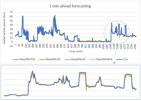
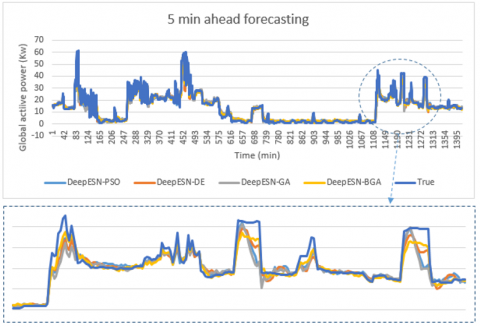
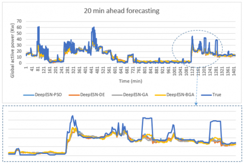
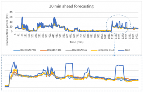
The result of this work, for four time horizons prediction (1 min, 5 min, 20 min, 30 min) are presented in Figures 7, 8, 9, and 10. In addition, the values of evaluation metrics error according to different time horizon prediction illustrated in Tables 4 and 5. Based on his ability to select the best architectures hyperparameters (Table 3), DeepESN-BGA has very interesting accuracy in term of RMSE, MSE, and MAE compared with other models based on Table 4. From the same table, it can be seen that DeepESN predict better than ESN based on two errors metrics. In comparison, between Reservoirs computing methods and RNN methods, the results of LSTM, GRU, and simple RNN have a larger error than ESN and DeepESN, in very short term horizon (1 min, and 5 min), that because the characteristics of dealing with non-linearity in RC-RNN, and his sophistical algorithms. The poor results in term of performance are of MLP, due to his architecture, which did not have memory capacity. In terms of forecasting horizon, the accuracy reduces according to the augmentation of time horizon values as it illustrated in Table 5. Regarding to the training performance of the models, it can be seen in Figure 11 that ESN and DeepESN trained faster than RNN, LSTM, GRU and MLP, thanks to his specific architecture, which allows the computation more flexible. In addition, DeepESN-BGA has also a good time for processing compared with LSTM and GRU, according to the illustrated results in Figure 11.
Table 3. The best values of architecture hyperparameters of DeepESN chosen based optimization algorithms
|
|
Time-horizon |
Nl |
Nn |
|
DeepESN-PSO |
1 min |
5 |
47 |
|
5 min |
8 |
49 |
|
|
20 min |
9 |
50 |
|
|
30 min |
10 |
50 |
|
|
DeepESN-GA |
1 min |
7 |
47 |
|
5 min |
8 |
44 |
|
|
20 min |
7 |
44 |
|
|
30 min |
9 |
45 |
|
|
DeepESN-DE |
1 min |
7 |
30 |
|
5 min |
5 |
30 |
|
|
20 min |
6 |
38 |
|
|
30 min |
10 |
55 |
|
|
DeepESN-BGA |
1 min |
6 |
20 |
|
5 min |
5 |
25 |
|
|
20 min |
8 |
30 |
|
|
30 min |
8 |
32 |
Table 4. The results of the prediction models in each time horizon
|
|
Time horizon |
ESN |
DeepESN |
LSTM |
GRU |
RNN |
MLP |
DeepESN-BGA |
|
MSE |
1 min 5 min 20 min 30 min |
0.00062 0.0023 0.00498 0.00591 |
0.000684 0.002329 0.00494 0.005804 |
0.000596 0.00214 0.004709 0.00556 |
0.00062 0.00210 0.004621 0.005542 |
0.000653 0.00226 0.00485 0.005702 |
0.000632 0.00228 0.00486 0.005705 |
0.000558 0.002206 0.004841 0.005714 |
|
MAE |
1 min 5 min 20 min 30 min |
0.01135 0.0259 0.0422 0.04853 |
0.01238 0.02511 0.042061 0.047844 |
0.01028 0.02331 0.04015 0.04698 |
0.01111 0.02272 0.03969 0.04696 |
0.01226 0.0236 0.04036 0.04638 |
0.0113 0.02396 0.0403 0.04655 |
0.00941 0.024071 0.041913 0.047344 |
|
RMSE |
1 min 5 min 20 min 30 min |
0.02507 0.0498 0.07057 0.07692 |
0.02616 0.04809 0.0703 0.07618 |
0.02441 0.04635 0.0686 0.074592 |
0.02523 0.04587 0.067978 0.07445 |
0.02556 0.047564 0.069669 0.075516 |
0.02515 0.04782 0.0697 0.075535 |
0.02363 0.04697 0.06958 0.07559 |
Table 5. The results of optimized model's prediction in each time horizon
|
|
Time horizon |
DeepESN-PSO |
DeepESN-DE |
DeepESN-GA |
DeepESN-BGA |
|
MSE |
1 min 5 min 20 min 30 min |
0.000553 0.002201 0.004831 0.005705 |
0.00057 0.00241 0.00499 0.00619 |
0.00056 0.00235 0.00489 0.00614 |
0.000558 0.002206 0.004841 0.005714 |
|
MAE |
1 min 5 min 20 min 30 min |
0.00932 0.02403 0.04182 0.04721 |
0.00948 0.02419 0.04923 0.04736 |
0.00946 0.02408 0.04191 0.04734 |
0.00941 0.02407 0.04191 0.04734 |
|
RMSE |
1 min 5 min 20 min 30 min |
0.02361 0.04692 0.06949 0.07545 |
0.02371 0.04699 0.06961 0.07562 |
0.02365 0.046 0.06958 0.07559 |
0.02363 0.04697 0.06958 0.07559 |
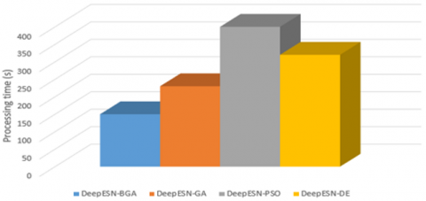
In term of optimization algorithms comparison, it can be seen that the values of hyperparameters are selected optimally to find the minimum fitness function by using BGA. It outperforms some comparative methods (GA and DE) based on their accuracies as it can be illustrated in Figures 11, 12, 13, 14 and Table 5. DeepESN-PSO has achieve good results especially in long term forecasting. However, PSO takes a long time in processing to select the best hyperparameters values.
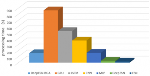
Figure 15 and 16 shows the time processing of each prediction model. As can be seen in Figure 15, the fastest model in terms of computation time is the ESN, while the slowest is the GRU. The proposed model, even when coupled with a BGA, is still better than GRU, LSTM and RNN. In Figure 16, hybridization with BGA outperforms that with other optimization models. Due to his binary characteristic BGA that lead to achieve best solution rapidly compared with others. These results indicate that the proposed model statistically has very interesting results, which make it a powerful method in the field of short-term power prediction.
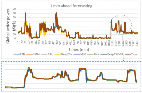
Figure 7. The comparison between prediction methods and true values for 1 min time horizon
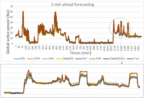
Figure 8. The comparison between prediction methods and true values for 5 min time horizon
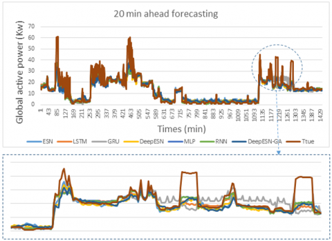
Figure 9. The comparison between prediction methods and true values for 20 min time horizon
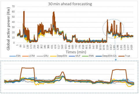
Figure 10. The comparison between prediction methods and true values for 30 min time horizon
Figure 11. The comparison between optimized Deep-ESNs and true values for 1 min time horizon
Figure 12. The comparison between optimized Deep-ESNs and true values for 5 min time horizon
A new combination between DeepESN and BGA are developed in this work, for obtaining an enhanced optimization models to predict a multi time horizon of household consumption in Paris, based on multivariate input. The performance of our proposed model is validated by analyzing the result of best hyperparameters using BGA, and comparing the accuracy and time training of different deep learning models. By combining DeepESN with BGA, the proposed method contains three advantages: Firstly, the property of basic ESN, which can deal properly with nonlinearity of time series, secondly the strong efficiency of deep learning computation, thirdly the ability to select the best and adequate architecture hyperparameters of the model. In all time horizons, the DeepESN-BGA has an excellent result in terms of accuracy compared to GRU, LSTM, RNN, MLP, ESN and DeepESN models. In addition, proposed model outperforms some of hybrid model as DeepESN-GA and DeepESN-DE in term of accuracy, especially in short term forecasting, by selecting best architecture hyperparameters. It can be seen also that the DeepESN-PSO predict better than proposed model in difference time horizon, but its processing takes a long time to find the best values of the hyperparameters. In the other hand, BGA has the fast computing processing compared with PSO, GA, and DE. With respect to all these results, DeepESN-BGA models achieved a high level of energy consumption forecasting in different time horizons, especially in the very short term. In addition, the combination of DeepESN and BGA is used for the first time in the literature. This gives it a new contribution in the field of deep learning prediction. Specifically, it is a new method to predict consumption energy for smart grid application.
In future work, the proposed models can be used for the prediction of energy production, and consumption price, and then this prediction will be used to manage the operation of the micro-grid in real time, by implementing the prediction model in hardware-embedded systems.
Figure 13. The comparison between optimized Deep-ESNs and true values for 20 min time horizon
Figure 14. The comparison between optimized Deep-ESNs and true values for 30 min time horizon
Figure 15. Processing time of different prediction models
Figure 16. Processing time of different optimized prediction models
[1] Boussetta, M., El Bachtiri, R., Khanfara, M., El Hammoumi, K. (2017). Assessing the potential of hybrid PV-wind systems to cover public facilities loads under different moroccan climate conditions. Sustainable Energy Technologies and Assessments, 22: 74-82. https://doi.org/10.1016/j.seta.2017.07.005
[2] Motahhir, S., Chalh, A., El Ghzizal, A., Derouich, A. (2018). Development of a low-cost PV system using an improved INC algorithm and a PV panel Proteus model. Journal of Cleaner Production, 204: 355-365. https://doi.org/10.1016/j.jclepro.2018.08.246
[3] https://www.bp.com/en/global/corporate/energy-economics/statistical-review-ofworld energy.html
[4] Konstantinou, C. (2022). Toward a secure and resilient all-renewable energy grid for smart cities. IEEE Consumer Electronics Magazine, 11(1): 33-41. https://doi.org/10.1109/MCE.2021.3055492
[5] Chaibi, Y., Allouhi, A., Salhi, M., El-jouni, A. (2019). Annual performance analysis of different maximum power point tracking techniques used in photovoltaic systems. Protection and Control of Modern Power Systems, 4(1): 1-10. https://doi.org/10.1186/s41601-019-0129-1
[6] Allouhi, A. (2020). Management of photovoltaic excess electricity generation via the power to hydrogen concept: A year-round dynamic assessment using Artificial Neural Networks. International Journal of Hydrogen Energy, 45(41): 21024-21039. https://doi.org/10.1016/j.ijhydene.2020.05.262
[7] Akhter, M.N., Mekhilef, S., Mokhlis, H., Shah, N.M. (2019). Review on forecasting of photovoltaic power generation based on machine learning and metaheuristic techniques. IET Renewable Power Generation, 13(7): 1009-1023. https://doi.org/10.1049/ietrpg.2018.5649
[8] Pappas, S.S., Ekonomou, L., Karamousantas, D.C., Chatzarakis, G.E., Katsikas, S.K., Liatsis, P. (2008). Electricity demand loads modeling using AutoRegressive Moving Average (ARMA) models. Energy, 33(9): 1353-1360. https://doi.org/10.1016/j.energy.2008.05.008
[9] Fan, J., Wang, X., Wu, L., Zhou, H., Zhang, F., Yu, X., Xiang, Y. (2018). Comparison of Support Vector Machine and Extreme Gradient Boosting for predicting daily global solar radiation using temperature and precipitation in humid subtropical climates: A case study in China. Energy Conversion and Management, 164: 102-111. https://doi.org/10.1016/j.enconman.2018.02.087
[10] Das, U.K., Tey, K.S., Seyedmahmoudian, M., Mekhilef, S., Idris, M.Y.I., Van Deventer, W., Stojcevski, A. (2018). Forecasting of photovoltaic power generation and model optimization: A review. Renewable and Sustainable Energy Reviews, 81: 912-928. https://doi.org/10.1016/j.rser.2017.08.017
[11] Tang, P., Chen, D., Hou, Y. (2016). Entropy method combined with extreme learning machine method for the short-term photovoltaic power generation forecasting. Chaos, Solitons and Fractals, 89: 243-248. https://doi.org/10.1016/j.chaos.2015.11.008
[12] Bendali, W., Saber, I., Boussetta, M., Mourad, Y., Bourachdi, B., Bossoufi, B. (2020). Deep learning for very short term solar irradiation forecasting. 2020 5th International Conference on Renewable Energies for Developing Countries (REDEC), Marrakech, Morocco, pp. 1-6. https://doi.org/10.1109/REDEC49234.2020.9163897
[13] Škrjanc, I., Iglesias, J., Sanchis, A., Leite, D., Lughofer, E., Gomide, F. (2019). Evolving fuzzy and neuro-fuzzy approaches in clustering, regression, identification, and classification: A survey. Information Sciences, 490: 344-368. https://doi.org/10.1016/j.ins.2019.03.060
[14] Bourbonnais R., Terraza M. (2008). Analyse de séries temporelles en économie, Paris, Dunod, 318 pages.
[15] Das, U.K., Tey, K.S., Seyedmahmoudian, M., Mekhilef, S., Idris, M.Y.I., Van Deventer, W., Stojcevski, A. (2018). Forecasting of photovoltaic power generation and model optimization: A review. Renewable and Sustainable Energy Reviews, 81: 912-928. https://doi.org/10.1016/j.rser.2017.08.017
[16] Hong, Y., Martinez, J.J., Fajardo, A.C. (2020). Day-ahead solar irradiation forecasting utilizing gramian angular field and convolutional long short-term memory. IEEE Access, 8: 18741-18753. https://doi.org/10.1109/ACCESS.2020.2967900
[17] Wojtkiewicz, J., Hosseini, M., Gottumukkala, R., Chambers, T.L. (2019). Hour-ahead solar irradiance forecasting using multivariate gated recurrent units. Energies, 12(21): 4055. https://doi.org/10.3390/en12214055
[18] Chembo, Y.K. (2020). Machine learning based on reservoir computing with time-delayed optoelectronic and photonic systems. Chaos: An Interdisciplinary Journal of Nonlinear Science, 30(1): 013111. https://doi.org/10.1063/1.5120788
[19] Hu, H., Wang, L., Lv, S.X. (2020). Forecasting energy consumption and wind power generation using deep echo state network. Renewable Energy, 154: 598-613. https://doi.org/10.1016/j.renene.2020.03.042
[20] Kiran, B.R., Sobh, I., Talpaert, V., Mannion, P., Sallab, A.A., Yogamani, S., Pérez, P. (2022). Deep reinforcement learning for autonomous driving: A survey. IEEE Transactions on Intelligent Transportation Systems, 23(6): 4909-4926. https://doi.org/10.1109/TITS.2021.3054625
[21] Nikita, S., Tiwari, A., Sonawat, D., Kodamana, H., Rathore, A.S. (2020). Reinforcement learning based optimization of process chromatography for continuous processing of biopharmaceuticals. Chemical Engineering Science, 230: 116171. https://doi.org/10.1016/j.ces.2020.116171
[22] Raviv, E., Bouwman, K.E., van Dijk, D. (2015). Forecasting day-ahead electricity prices: utilizing hourly prices. Energy Economics, 50: 227-239. https://doi.org/10.1016/j.eneco.2015.05.014
[23] Bendali, W., Saber, I., Bourachdi, B., Amri, O., Boussetta, M., Mourad, Y. (2022). Multi time horizon ahead solar irradiation prediction using GRU, PCA, and GRID SEARCH based on multivariate datasets. Journal Européen des Systèmes Automatisés, 55(1): 11-23. https://doi.org/10.18280/jesa.550102
[24] Amarasinghe, K., Marino, D.L., Manic, M. (2017). Deep neural networks for energy load forecasting. 2017 IEEE 26th International Symposium on Industrial Electronics (ISIE), Edinburgh, UK, pp. 1483-1488. https://doi.org/10.1109/ISIE.2017.8001465
[25] Grolinger, K., L’Heureux, A., Capretz, M.A., Seewald, L. (2016). Energy forecasting for event venues: Big data and prediction accuracy. Energy and Buildings, 112: 222-233. https://doi.org/10.1016/j.enbuild.2015.12.010
[26] Saez-Gallego, J., Morales, J.M., Zugno, M., Madsen, H. (2016). A data-driven bidding model for a cluster of priceresponsive consumers of electricity. IEEE Transactions on Power Systems, 31(6): 5001-5011. https://doi.org/10.1109/TPWRS.2016.2530843
[27] Browne, M.W. (2000). Cross-validation methods. Journal of Mathematical Psychology, 44(1): 108-132. https://doi.org/10.1006/jmps.1999.1279
[28] Saleh, A.I., Rabie, A.H., Abo-Al-Ez, K.M. (2016). A data mining based load forecasting strategy for smart electrical grids. Advanced Engineering Informatics, 30(3): 422-448. https://doi.org/10.1016/j.aei.2016.05.005
[29] Lago, J., Ridder, F.D., Vrancx, P., Schutter, B.D. (2018). Forecasting day-ahead electricity prices in Europe: The importance of considering market integration. Applied Energy, 211: 890-903. https://doi.org/10.1016/j.apenergy.2017.11.098
[30] Khalid, R., Javaid, N. (2020). A Survey on Hyperparameters Optimization Algorithms of Forecasting Models in Smart Grid. Sustainable Cities and Society, 61: 102275. https://doi.org/10.1016/j.scs.2020.102275
[31] González, J.P., Roque, A.M., Pérez, E.A. (2018). Forecasting functional time series with a new hilbertian ARMAX model: Application to Electricity Price Forecasting. IEEE Transactions on Power Systems, 33(1): 545-556. https://doi.org/10.1109/TPWRS.2017.2700287
[32] Sulaiman, S., Jeyanthy, P.A., Devaraj, D. (2016). Big data analytics of smart meter data using adaptive neuro fuzzy inference system (ANFIS). 2016 International Conference on Emerging Technological Trends (ICETT), Kollam, India, pp. 1-5. https://doi.org/10.1109/ICETT.2016.7873732
[33] Chitsaz, H., Shaker, H.R., Zareipour, H., Wood, D.H., Amjady, N. (2015). Short-term electricity load forecasting of buildings in microgrids. Energy and Buildings, 99: 50-60. https://doi.org/10.1016/j.enbuild.2015.04.011
[34] Sheng, G., Hou, H., Jiang, X., Chen, Y. (2018). A Novel Association Rule Mining Method of Big Data for Power Transformers State Parameters Based on Probabilistic Graph Model. IEEE Transactions on Smart Grid, 9(2): 695-702. https://doi.org/10.1109/TSG.2016.2562123
[35] Yue, M., Toto, T., Jensen, M.P., Giangrande, S.E., Lofaro, R. (2018). A Bayesian Approach-Based Outage Prediction in Electric Utility Systems Using Radar Measurement Data. IEEE Transactions on Smart Grid, 9: 6149-6159. https://doi.org/10.1109/TSG.2017.2704288
[36] Yu, C., Mirowski, P.W., Ho, T.K. (2017). A Sparse Coding Approach to Household Electricity Demand Forecasting in Smart Grids. IEEE Transactions on Smart Grid, 8(2): 738-748. https://doi.org/10.1109/TSG.2015.2513900
[37] Aslam, S., Khalid, A., Javaid, N. (2020). Towards efficient energy management in smart grids considering microgrids with day-ahead energy forecasting. Electric Power Systems Research, 182: 106232. https://doi.org/10.1016/j.epsr.2020.106232
[38] Zhou, Z., Xiong, F., Huang, B., Xu, C., Jiao, R., Liao, B., Yin, Z., Li, J. (2017). Game-theoretical energy management for energy internet with big data-based renewable power forecasting. IEEE Access, 5: 5731-5746. https://doi.org/10.1109/ACCESS.2017.2658952
[39] Bendali, W., Saber, I., Bourachdi, B., Boussetta, M., Mourad, Y. (2020). Deep learning using genetic algorithm optimization for short term solar irradiance forecasting. 2020 Fourth International Conference On Intelligent Computing in Data Sciences (ICDS), Fez, Morocco, pp. 1-8. https://doi.org/10.1109/ICDS50568.2020.9268682
[40] Alamaniotis, M., Bargiotas, D., Bourbakis, N.G., Tsoukalas, L.H. (2015). Genetic optimal regression of relevance vector machines for electricity pricing signal forecasting in smart grids. IEEE Transactions on Smart Grid, 6(6): 2997-3005. https://doi.org/10.1109/TSG.2015.2421900
[41] Raza, M.Q., Nadarajah, M., Ekanayake, C. (2017). Demand forecast of PV integrated bioclimatic buildings using ensemble framework. Applied Energy, 208: 1626-1638. https://doi.org/10.1016/j.apenergy.2017.08.192
[42] Xiao, L., Wang, J., Hou, R., Wu, J. (2015). A combined model based on data pre-analysis and weight coefficients optimization for electrical load forecasting. Energy, 82: 524-549. https://doi.org/10.1016/j.energy.2015.01.063
[43] Kavousi-Fard, A., Samet, H., Marzbani, F. (2014). A new hybrid modified firefly algorithm and support vector regression model for accurate short term load forecasting. Expert Systems with Applications, 41(13): 6047-6056. https://doi.org/10.1016/j.eswa.2014.03.053
[44] Shayeghi, H., Ghasemi, A., Moradzadeh, M., Nooshyar, M. (2015). Simultaneous day-ahead forecasting of electricity price and load in smart grids. Energy Conversion and Management, 95: 371-384. https://doi.org/10.1016/j.enconman.2015.02.023
[45] Liu, Y., Wang, W., Ghadimi, N. (2017). Electricity load forecasting by an improved forecast engine for building level consumers. Energy, 139: 18-30. https://doi.org/10.1016/j.energy.2017.07.150
[46] Chou, J., Ngo, N. (2016). Smart grid data analytics framework for increasing energy savings in residential buildings. Automation in Construction, 72(3): 247-257. https://doi.org/10.1016/j.autcon.2016.01.002
[47] Khalid, R., Javaid, N., Al-Zahrani, F.A., Aurangzeb, K., Qazi, E., Ashfaq, T. (2020). Electricity load and price forecasting using jaya-long short term memory (JLSTM) in smart grids. Entropy, 22(1): 10. https://doi.org/10.3390/e22010010
[48] Singh, N., Mohanty, S.R., Shukla, R.D. (2017). Short term electricity price forecast based on environmentally adapted generalized neuron. Energy, 125: 127-139. https://doi.org/10.1016/j.energy.2017.02.094
[49] Young, S.R., Rose, D.C., Karnowski, T.P., Lim, S.H., Patton, R.M. (2015). Optimizing deep learning hyper-parameters through an evolutionary algorithm. Proceedings of the Workshop on Machine Learning in High-Performance Computing Environments - MLHPC ’15. https://doi.org/doi:10.1145/2834892.2834896
[50] Lonij, V.P., Brooks, A.E., Cronin, A.D., Leuthold, M., Koch, K. (2013). Intra-hour forecasts of solar power production using measurements from a network of irradiance sensors. Solar Energy, 97: 58-66. https://doi.org/10.1016/j.solener.2013.08.002
[51] Li, H., Cao, J.N., Love, P.E.D. (1999). Using machine learning and GA to solve time-cost trade-off problems. Journal of Construction Engineering and Management, 125(5): 347-353. https://doi.org/10.1061/(asce)0733-9364(1999)125:5(347)
[52] Tanaka, G., Yamane, T., Héroux, J.B., Nakane, R., Kanazawa, N., Takeda, S., Numata, H., Nakano, D., Hirose, A. (2019). Recent advances in physical reservoir computing: A review. Neural networks: The official Journal of the International Neural Network Society, 115: 100-123. https://doi.org/10.1016/j.neunet.2019.03.005
[53] Chouikhi, N., Ammar, B., Rokbani, N., Alimi, A.M. (2017). PSO-based analysis of echo state network parameters for time series forecasting. Applied Soft Computing, 55: 211-225. https://doi.org/10.1016/j.asoc.2017.01.049
[54] Ma, Q., Shen, L., Chen, W., Wang, J., Wei, J., Yu, Z. (2016). Functional echo state network for time series classification. Information Sciences, 373: 1-20. https://doi.org/10.1016/j.ins.2016.08.081
[55] Wang, L., Hu, H., Ai, X.Y., Liu, H. (2018). Effective electricity energy consumption forecasting using echo state network improved by differential evolution algorithm. Energy, 153: 801-815. https://doi.org/10.1016/j.energy.2018.04.078
[56] Chitsazan, M.A., Sami Fadali, M., Trzynadlowski, A.M. (2019). Wind speed and wind direction forecasting using echo state network with nonlinear functions. Renewable Energy, 131: 879-889. https://doi.org/10.1016/j.renene.2018.07.060
[57] Balakrishnan, M., Tv, G. (2020). A neural network framework for predicting dynamic variations in heterogeneous social networks. Plos One, 15(4): e0231842. https://doi.org/10.1371/journal.pone.0231842
[58] Gallicchio, C., Micheli, A., Pedrelli, L. (2017). Deep reservoir computing: A critical experimental analysis. Neurocomputing, 268: 87-99. https://doi.org/10.1016/j.neucom.2016.12.089
[59] Bilgili, M.S., Şahin, B., Yaşar, A., Şimşek, E. (2012). Electric energy demands of Turkey in residential and industrial sectors. Renewable & Sustainable Energy Reviews, 16(1): 404-414. https://doi.org/10.1016/j.rser.2011.08.005
[60] Jaeger, H. (2001). Short term memory in echo state networks. Technical report, German National Research Center for Information Technology, Germany.
[61] Gallicchio, C., Micheli, A. (2017). Echo state property of deep reservoir computing networks. Cognitive Computation, 9(3): 337-350. https://doi.org/10.1007/s12559-017-9461-9
[62] Gallicchio, C., Micheli, A. (2017). Deep echo state network (DeepESN): A brief survey. ArXiv. https://doi.org/10.48550/arXiv.1712.04323
[63] Kim, J., Yoo, S. (2019). Software review: Deap (distributed evolutionary algorithm in python) library. Genetic Programming and Evolvable Machines, 20(1): 139-142. https://doi.org/10.1007/s10710-018-9341-4
[64] Bejan, A. (2016). Constructal thermodynamics. International Journal of Heat and Technology, 34: S1-S8. https://dx.doi.org/10.18280/ijht.34S101
[65] Berard, A. (2012). TELECOM ParisTech Master of Engineering Internship at EDF R&D, Clamart, France. https://archive.ics.uci.edu/ml/datasets/individual+household+electric+power+consumption