A Non-Cooperative Distributed Model Predictive Control Using Laguerre Functions for Large-Scale Interconnected Systems

Let a discrete-time linear and time-invariant global system be given by

$\mathcal{S}= \begin{cases}\mathrm{x}_{(k+1)} & =A \mathrm{x}_{(k)}+B \mathrm{u}_{(k)} \\ \mathrm{y}_{(k)} & =C \mathrm{x}_{(k)}\end{cases}$      (1)

where, $\mathrm{x}_{(k)} \in \Re^{n_x}$ is the state of the system, $\mathrm{u}_{(k)} \in \mathfrak{R}^{n_u}$ is its input and $\mathrm{y}_{(k)} \in \mathfrak{R}^{n_y}$ is its output with $k>0$ an integer index denoting discrete time. The whole system matrices are $A \in$ $\mathfrak{R}^{n_x \times n_x}, B \in \Re^{n_x \times n_u}$ and $C \in \Re^{n_y \times n_x}$. Consider the decoupled subplants or decentralized models derived from (1),

$\mathcal{S}_{i i}= \begin{cases}\mathrm{x}_{(k+1)}^{\{i\}} & =A_{i i} \mathrm{x}_{(k)}^{\{i\}}+B_{i i} \mathrm{u}_{(k)}^{\{i\}} \\ \mathrm{y}_{(k)}^{\{i\}} & =C_{i i} \mathrm{x}_{(k)}^{\{i\}} \quad i=\overline{1, \mathbb{N}}\end{cases}$        (2)

where, vectors $x_{(k)}^{\{i\}} \in \mathfrak{R}^{n_{x_i}}, \mathrm{u}_{(k)}^{\{i\}} \in \mathfrak{R}^{n_{u_i}}$ are the local states and inputs, respectively, of the $i^{t h}$ subsystem, while $y_{(k)}^{\{i\}} \in$ $\mathfrak{R}^{n_{y_i}}$ is its local output. The dimensions of these local vectors are such that

$n_x=\sum_{i=1}^{\mathbb{N}} n_{x_i}, n_u=\sum_{i=1}^{\mathbb{N}} n_{u_i}, n_y=\sum_{i=1}^{\mathbb{N}} n_{y_i}$

and the global state vector can be written as $\mathrm{x}=\operatorname{col}_{i \in\{1, \ldots, \mathbb{N}\}}\quad\left(\mathrm{x}^{\{i\} }\right),\left(\xi=\operatorname{col}_{i \in\{1, \ldots, \mathbb{N}\}}\quad\left(\xi^{\{i\}}\right)\right.$: vector consisting of stacked subvectors $\left.\xi^{\{i\} \quad}\right)$, the global input as $\mathrm{u}=\operatorname{col}_{i \in\{1, \ldots, \mathbb{N}\}}\quad\left(\mathrm{u}^{\{i\} }\right)$, the global output as $y=\operatorname{col}_{i \in\{1, \ldots, \mathbb{N}\}}\quad\left(y^{\{i\}}\right)$. Note that the interconnected system’s elements are generally strongly coupled. Consequently, the decentralized control design leads to poor performance requirements or even instability because it has not the potential to take into account these interactions between the subsystems.

Throughout this manuscript, we suppose that the global system $\mathcal{S}$ in (1) is composed of $\mathbb{N}$ subsystems $\mathcal{S}_i$. Therefore, any subsystem $\mathcal{S}_i$ can be interacting with the other subsystems $\mathcal{S}_j, j \neq i$ through linear interconnections. Therefore, the local dynamics of any subsystem $\mathcal{S}_i, i=\overline{1, \mathbb{N}}$, is described as follows:

$S_i= \begin{cases}\mathrm{x}_{(k+1)}^{\{i\}} & =A_{i i} \mathrm{x}_{(k)}^{\{i\}}+B_{i i} \mathrm{u}_{(k)}^{\{i\}}+\sum_{j=1}^{\mathbb{N}}\left[A_{i j} \mathrm{x}_{(k)}^{\{j\}}+B_{i j} \mathrm{u}_{(k)}^{\{j\}}\right] \\ \mathrm{y}_{(k)}^{\{i\}} & =C_{i i} \mathrm{x}_{(k)}^{\{i\}}+\sum_{j=1}^{\mathbb{N}} C_{i j} \mathrm{x}_{(k)}^{\{j\}} \quad i=\overline{1, \mathbb{N}}, j \neq i\end{cases}$        (3)

The interaction vectors are built upon state and input interactions produced on the subsystem $\mathcal{S}_i$ by the other subsystems $\mathcal{S}_j, j \neq i$ are described as follows:

$\mathrm{v}_{(k)}^{\{i\}}=\sum_{j=1}^{\mathbb{N}}\left[A_{i j} \mathrm{x}_{(k)}^{\{j\}}+B_{i j} \mathrm{u}_{(k)}^{\{j\}}\right]$

$\mathrm{w}_{(k)}^{\{i\}}=\sum_{j=1}^{\mathbb{N}} C_{i j} \mathrm{x}_{(k)}^{\{j\}}$      (4)

According to this representation, the matrices $A_{i j}, B_{i j}$ and $C_{i j}$, for $i \neq j$, define the dynamic coupling terms between the subsystems.

In general, not all the subsystems might have an influence on each other. To account for the influences between the subsystems, let us introduce the following definition

Definition 1 A subsystem $\mathcal{S}_j$ interacts dynamically with the subsystem $\mathcal{S}_i$ if and only if, at least, one of the matrices $A_{i j}, B_{i j}, C_{i j}$ is non null, i.e., if and only if the states $x^{\{j\}}$ and/or inputs $u^{\{j\}}$ of $\mathcal{S}_j$ affect the dynamics of $\mathcal{S}_i$.

1.png

(a) Centralized control

1b.png

(b) Decentralized control

1c.png

(c) Distributed control

Figure 1. A schematic illustration of the principal control system architectures

The distributed control architecture dealed with throughout the paper has the generic structure given in Figure 1(c). This architecture consists of several local controllers, each dedicated to a subsystem of the overall plant, which can exchange information over a digital communication network. This architecture favors a non-cooperation based control strategy for large-scale interconnected systems (3)-(4) that aims to emulate the performance achievable with a centralized control scheme of Figure 1(a).

In a typical DMPC framework, $\mathbb{N}$ subproblems are resolved, each one assigned to different sub-controllers $\mathcal{C}_i, i=\overline{1, \mathbb{N}}$, instead of a single centralized problem.

The following procedure achieved by the set of independent local controllers $\mathcal{C}_i$, at each time instant $k$, is given by: 1 ) acquire both local output measurements on $\mathcal{S}_i$ and the received estimate of the interactions between $\mathcal{S}_i$ and the other subsystems $\mathcal{S}_j, j=\overline{1, \mathbb{N}}, j \neq i$, transmitted through the communication network, to predicate the local state variable over the prediction horizon, 2) resolve the local optimization problem, 3) calculate the first control sample and apply it as a control input, 4) share both local optimal control sequence and future state prediction information with the other controllers through the communication network.

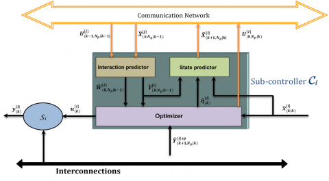
In DMPC formulation, the whole-size optimization problem is replaced by $\mathbb{N}$ small sub-problems working together towards achieving the best performance of the centralized control system. To obtain an explicit solution of the work on the nominal distributed optimization problem presented by Vaccarini et al. [12, 13], each sub-controller $\mathcal{C}_i$ is composed of three parts: an optimizer, a state predictor and an interaction predictor (see Figure 3). The workflow of each sub-controller will be described later in algorithmic form in section 7.

For the sake of simplicity, the availability of the local states $\hat{x}_{(k)}^{\{i\}}$  through measurements is assumed. Furthermore, denoting  $N_{p i}$  and $N_{u i}$  the prediction and control horizons for the $i^{t h}$  sub-controller  $\mathcal{C}_i$, the subsequent assumptions are adopted in the sequel:

Assumptions 1

a. the prediction and control horizons are equal, i.e., $N_p=N_{p_i}=N_{p_j}$ and $N_u=N_{u_i}=N_{u_j}, \forall j, i=\overline{1, \mathbb{N}}, i \neq j$;

b. the sub-controllers $\mathcal{C}_i$, for $i=\overline{1, \mathbb{N}}$, act in a synchronous way;

c. the information is transmitted (and received) by the local sub-controllers only once within each sampling time interval (non-iterative algorithm);

d. the digital network introduces one step communication delay;

e. the information exchange is not loosed during the transmission;

f. all the pairs $\left(A_{i i}, B_{i i}\right)$ are stabilizable.

At each time instant $k$, neither $\mathrm{x}_{(k)}^{\{j\}}$ nor $\mathrm{u}_{(k)}^{\{j\}}$ for $j \neq i$ are available by the agent $\mathcal{C}_i$; only their predictions, previously sent by the agents $\mathcal{C}_j$, are known. In fact, due to the unit delay introduced by the communication network (cf. Assumption 1-(d) above), the information of the other subsystems is available only after one sampling time interval. Therefore, the interaction predictions $\widehat{\mathrm{v}}_{(k+l-s \mid k)}^{\{i\}}$ and $\widehat{\mathrm{w}}_{(k+l-s \mid k)}^{\{i\}}$ are unavailable at current time $k$ for the subsystem $\mathcal{S}_i$. Then, theirs values are available after one sampling time interval with respect to the instant they are broadcasted in. For this reason, the predictions $\hat{\mathrm{v}}_{(k+l-s \mid k-1)}^{\{i\}}$ and $\widehat{\mathrm{w}}_{(k+l-s \mid k-1)}^{\{i\}}$ will be used instead of $\hat{\mathrm{v}}_{(k+l-s \mid k)}^{i\}}$ and $\widehat{\mathrm{w}}_{(k+l-s \mid k)}^{\{i\}}$ in the subsequent problem definition.

For mathematical notation simplicity, the following notations are used in this paper:

• $\operatorname{diag}_\alpha[\Lambda]=$ block-diag $\{\underbrace{\Lambda \Lambda \ldots \Lambda}_{\alpha \text { times }}\}$;

• $0_{\alpha \times \beta}\left(I_{\alpha \times \beta}\right)$ is the null (identity) matrix in $\mathfrak{R}^{\alpha \times \beta}$;

• $0_\alpha\left(I_\alpha\right)$ is the null (identity) matrix in $\Re^{\alpha \times \alpha}$;

• 0 is the null matrix or vector with appropriate dimensions.

4.1 State predictor

The l-step ahead predicted state variable of the $i^{t h}$ subsystem, at each time instant k, is given by:

$\hat{\mathrm{x}}_{(k+l \mid k)}^{\{i\}}=A_{i i}^l \hat{\mathrm{x}}_{(k \mid k)}^{\{i\}}+\sum_{s=1}^l\left[A_{i i}^{s-1} B_{i i} \mathrm{u}_{(k+l-s \mid k)}^{\{i\}}+A_{i i}^{s-1} \hat{\mathrm{v}}_{(k+l-s \mid k-1)}^{\{i\}}\quad\right]$   (7)

where, $\hat{\mathrm{v}}_{(k+l-s \mid k-1)}^{\{i\}}$ denotes the prediction of $\mathrm{v}_{(k+l-s)}^{\{i\}}$ computed at the past time instant $k-1$.

4.2 Interaction prediction

The interaction predictions of the $i^{t h}$ subsystem, at each time instant k, are expressed as follows :

$\begin{aligned} \hat{\mathcal{V}}_{\left(k, N_p \mid k-1\right)}^{\{i\}} & =\tilde{A}_i \widehat{\mathrm{X}}_{\left(k, N_p \mid k-1\right)}+\tilde{B}_i \tilde{\Gamma}_i \mathrm{U}_{\left(k-1, N_u \mid k-1\right)} \\ \widehat{\mathcal{W}}_{\left(k, N_p \mid k-1\right)}^{\{i\}} & =\tilde{C}_i \widehat{\mathrm{X}}_{\left(k, N_p \mid k-1\right)}\end{aligned}$      (8)

Now, let us assume that:

$\widetilde{K}_i=\left[\operatorname{diag}_p\left(K_{i 1}\right) \ldots \operatorname{diag}_p\left(K_{i i-1}\right) 0 \operatorname{diag}_p\left(K_{i i+1}\right) \ldots \operatorname{diag}_p\left(K_{i \mathbb{N}}\right)\right]$

with $\widetilde{K}_i \in\left\{\tilde{C}_i, \tilde{B}_i, \tilde{A}_i\right\}$

4.3 Optimal control sequence of each independent sub-controller C_i

At each sampling time instant $k$, when a set of the estimation vectors $\widehat{X}^{\{j\}}$ and $\mathrm{U}^{\{j\}}$ are received from the other sub-controllers $\mathcal{C}_j, j=\overline{1, \mathbb{N}}, j \neq i$ through the communication network (cf. Assumption 1-(d) above), the interaction predictor of each independent $\mathcal{C}_i$ uses these information to estimate the interaction predictions. Then, these predictions are gathered with the local state value $x_{(k)}^{\{i\}}$ and all these information to be used by the optimizer in order to find a solution of the local optimization problem. Once the sequence of future control values $\Delta \mathrm{U}^{*\{i\}}=\left\{\Delta \mathrm{u}_{(k \mid k)}^{*\{i\}}, \ldots, \Delta \mathrm{u}_{\left(k+N_u-1 \mid k\right)}^{*\{i\}}\right\}$ is computed by solving the finite-horizon optimal control problem (6), only the first sample of the computed optimal control sequence is retained and $\mathrm{u}_{(k \mid k)}^{*\{i\}}=\Delta \mathrm{u}_{(k \mid k)}^{*\{i\}}+\mathrm{u}_{(k-1)}^{*\{i\}}$ is injected as the control action to the subsystem $\mathcal{S}_i$, while neglecting the rest of the elements constituting the computed optimal sequence. At the same time, by means (7), the state predictor estimates the future state variable. Then, the optimal control sequence together with the state predictions over the prediction horizon $N_p$ are broadcasted to the other sub-controllers $\mathcal{C}_j, j \neq i$, through the communication network. At the next time instant, $k+1$, the overall procedure is repeated, for each local controller, according to the so-called receding horizon principle.

Usually, the horizons N_p and N_u are two important tuning parameters of the MPC control design. However, the computational burden in MPC is directly depending upon theme. Among the MPC formulations, the well known one is the classical scheme [38-40]. In this technique, for the possibility of high rapid sampling frequency, complex plant dynamics and/or high requirement on the global system performance, satisfactory approximation of the control increment $\Delta \mathrm{u}_{(k)}^{\{i\}}$ could involve a vast number of parameters (especially N_u), resulting in poorly numerically conditioned solutions with a weighty computational burden [41]. Otherwise, a more suitable approach is to use Laguerre functions [42, 43] in the design of MPC.

6.1 The modified interaction prediction 

Given the measurements until instant $h$, the future states, inputs and interactions vectors from instant $k$ to instant $k+l-1$, with $k \geq h$, are expressed by

$\widehat{\mathrm{D}}_{(k, l \mid h)}^{\{i\}}=\left[\begin{array}{l}\hat{\mathrm{d}}_{(k \mid h)}^{\{i\}} \\ \mathrm{d}_{(k+1 \mid h)}^{\{i)} \\ \vdots \\ \widehat{\mathrm{d}}_{(k+l-1 \mid h)}^{(i)}\end{array}\right], \widehat{\mathrm{D}}_{(k, l \mid h)}=\left[\begin{array}{l}\widehat{\mathrm{D}}_{(k, l \mid h)}^{\{1\}} \\ \widehat{\mathrm{D}}_{(k, l \mid h)}^{\{2\}} \\ \vdots \\ \widehat{\mathrm{D}}_{(k, l \mid h)}^{\{\mathbb{N}\}}\end{array}\right]$

where, $\widehat{\mathrm{d}} \in\{\hat{\mathrm{x}}, \hat{\mathrm{y}}, \widehat{\mathrm{w}}, \hat{\mathrm{v}}\}$ and $\widehat{\mathrm{D}} \in\{\widehat{\mathrm{X}}, \widehat{\mathrm{Y}}, \widehat{\mathcal{W}}, \hat{\mathcal{V}}\}$.

$\mathrm{U}_{(k, l \mid h)}^{\{i\}}=\left[\begin{array}{l}\mathrm{u}_{(k \mid h)}^{\{i\}} \\ \mathrm{u}_{(k+1 \mid h)}^{\{i\}} \\ \vdots \\ \mathrm{u}_{(k+l-1 \mid h)}^{\{i\}}\end{array}\right], \mathrm{U}_{(k, l \mid h)}=\left[\begin{array}{l}\mathrm{U}_{(k, l \mid h)}^{\{1\}} \\ \mathrm{U}_{(k, l \mid h)}^{\{2\}} \\ \vdots \\ \mathrm{U}_{(k, l \mid h)}^{\{\mathbb{N}\}}\end{array}\right]$

Furthermore, let us assume that: 

$\tilde{P}_i=\left[\begin{array}{lllllll}P_{i 1} & \ldots & P_{i i-1} & 0 & P_{i i+1} & \ldots & P_{i \mathbb{N}}\end{array}\right]$

where, $\tilde{P}_i \in\left\{\tilde{A}_i, \tilde{B}_i, \tilde{C}_i\right\}$.

For $i=\overline{1, \mathbb{N}}$, the $l$-step ahead predictions of the local interaction vectors, at time instant $k$, can be described as follows:

$\begin{aligned} \widehat{\mathrm{v}}_{(k+l \mid k)}^{\{i\}} & =\sum_{j=1(j \neq i)}^{\mathbb{N}}\left[A_{i j} \hat{\mathrm{x}}_{(k+l \mid k)}^{\{j\}}+B_{i j} \mathrm{u}_{(k+l \mid k)}^{\{j\}}\right] \\ \widehat{\mathrm{w}}_{(k+l \mid k)}^{\{i\}} & =\sum_{j=1(j \neq i)}^{\mathbb{N}} C_{i j} \hat{\mathrm{x}}_{(k+l \mid k)}^{\{j\}}\end{aligned}$       (19)

Using the previous definitions, the compact form of the interaction prediction vectors can be expressed as follows 

$\widehat{\mathcal{V}}_{\left(k, N_p \mid k-1\right)}^{\{i\}}=\tilde{A}_i \widehat{X}_{(k, N p \mid k-1)}+\tilde{B}_i \mathrm{U}_{\left(k, N_p \mid k-1\right)}$

$\widehat{\mathcal{W}}_{\left(k, N_p \mid k-1\right)}^{\{i\}}=\tilde{C}_i \widehat{X}_{\left(k, N_p \mid k-1\right)}$    (20)

Referring to Assumption 1-(d), the information of the other subsystems is available only after one sampling time interval. In this case, $\mathrm{U}_{\left(k, N_p \mid k-1\right)}^{\{i\}}$ and $\mathrm{U}_{\left(k, N_p \mid k-1\right)}$ can be expressed in terms of $\mathrm{U}_{\left(k-1, N_p \mid k-1\right)}^{\{i\}}$ and $\mathrm{U}_{\left(k-1, N_p \mid k-1\right)}$ respectively as follows:

$\mathrm{U}_{\left(k, N_p \mid k-1\right)}^{\{i\}}=\hat{\Gamma}_i \mathrm{U}_{\left(k-1, N_p \mid k-1\right)}^{\{i\}}$    (21a)

$\mathrm{U}_{\left(k, N_p \mid k-1\right)}=\hat{\Gamma} \mathrm{U}_{\left(k-1, N_p \mid k-1\right)}$    (21b)

where, 

00.png

$\hat{\Gamma}=\operatorname{diag}\left\{\hat{\Gamma}_1, \hat{\Gamma}_2, \ldots, \hat{\Gamma}_{\mathbb{N}}\right\}$

By substituting (21a) into (20), the interaction prediction vectors can be rewritten as follows:

$\widehat{\mathcal{V}}_{\left(k, N_p \mid k-1\right)}^{\{i\}}=\tilde{A}_i \widehat{X}_{\left(k, N_p \mid k-1\right)}+\tilde{B}_i \hat{\Gamma}_i \mathrm{U}_{\left(k-1, N_p \mid k-1\right)}$

$\widehat{\mathcal{W}}_{\left(k, N_p \mid k-1\right)}^{\{i\}}=\tilde{C}_i \widehat{X}_{\left(k, N_p \mid k-1\right)}$   (22)

Note that the state predictions and the control actions contained in expression (22) are calculated at time instant k-1 and transmitted through the digital network.

6.2 The modified state predictor

The state variable of the i^th subsystem, at sampling instant l, can be predicted as follows: 

$\hat{\mathrm{x}}_{(k+l \mid k)}^{\{i\}}=A_{i i}^l \hat{\mathrm{x}}_{(k \mid k)}^{\{i\}}+\sum_{s=1}^l A_{i i}^{s-1}\left[B_{i i} \mathrm{u}_{(k+l-s \mid k)}^{\{i\}}+A_{i i}^{s-1} \hat{\mathrm{v}}_{(k+l-s \mid k-1)}^{\{i\}}\quad\right]$    (23)

Let us now define, for $l=\overline{1, N_p}$

$\mathrm{u}_{(k+l-s \mid k)}^{\{i\}}=\mathrm{u}_{(k-1)}^{\{i\}}+\sum_{n=s}^l \Delta \mathrm{u}_{(k-s-1 \mid k)}^{\{i\}}$ for $s=\overline{1, l}$    (24)

By means (23) and (24), the states $\widehat{\mathrm{x}}_{(k+l \mid k)}^{\{i\}}$ become

$\hat{\mathrm{x}}_{(k+l \mid k)}^{\{i\}}=A_{i i}^l \hat{\mathrm{x}}_{(k \mid k)}^{\{i\}}+\sum_{s=1}^l A_{i i}^{s-1} B_{i i} \mathrm{u}_{(k-1)}^{\{i\}}$$+\sum_{s=1}^l\left(\sum_{n=s}^l A_{i i}^{l-n} B_{i i}\right) \Delta \mathrm{u}_{(k+s-1 \mid k)}^{\{i\}}$$+\sum_{s=1}^l A_{i i}^{s-1} \hat{\mathrm{v}}_{(k+l-s \mid k-1)}^{\{i\}}$    (25)

According to the expression (15), the incremental control trajectory along the prediction horizon at time instant $k$ can be calculated as $\Delta \mathrm{u}_{(k+s-1 \mid k)}^{\{i\}}=\mathcal{L}_{i(s-1)}^T \eta_i$ in Laguerre formulation.

Then, the l-step ahead states can be predicted by

$\hat{\mathrm{x}}_{(k+l \mid k)}^{\{i\}}=A_{i i}^l \hat{\mathrm{x}}_{(k \mid k)}^{\{i\}}+\sum_{s=1}^l A_{i i}^{s-1} B_{i i} \mathrm{u}_{(k-1)}^{\{i\}}$$+\sum_{s=1}^l\left(\sum_{n=s}^l A_{i i}^{l-n} B_{i i}\right) \mathcal{L}_{i(s-1)}^T \eta_i$$+\sum_{s=1}^l A_{i i}^{s-1} \widehat{\mathrm{v}}_{(k+l-s \mid k-1)}^{\{i\}}$    (26)

where, the predicted control is rewritten as

$\sum_{s=1}^l A_{i i}^{s-1} B_{i i} \mathrm{u}_{(k+l-s \mid k)}^{\{i\}}=$$=\sum_{s=1}^l A_{i i}^{s-1} B_{i i} \mathrm{u}_{(k-1)}^{\{i\}}$$+\sum_{s=1}^l\left(\sum_{n=s}^l A_{i i}^{l-n} B_{i i}\right) \mathcal{L}_{i(s-1)}^T \eta_i$

and the predicted output variable writes

$\hat{\mathrm{y}}_{(k+l \mid k)}^{\{i\}}=C_{i i} A_{i i}^l \hat{\mathrm{x}}_{(k \mid k)}^{\{i\}}+C_{i i} \sum_{s=1}^l A_{i i}^{s-1} B_{i i} \mathrm{u}_{(k-1)}^{\{i\}}$$+C_{i i} \sum_{s=1}^l\left(\sum_{n=s}^l A_{i i}^{l-n} B_{i i}\right) \mathcal{L}_{i(s-1)}^T \eta_i$$+C_{i i} \sum^l A_{i i}^{s-1} \widehat{\mathrm{v}}_{(k+l-s \mid k-1)}^{\{i\}}+\widehat{\mathrm{w}}_{(k+l \mid k-1)}^{\{i\}}$    (27)

The previous expressions of the predicted future state and output variables, show that the control signal $\mathrm{u}_{(k)}^{\{i\}}$ is not needed and it can be replaced by the coefficient vector $\eta_i$. However, the main idea is finding the coefficient vector $\eta_i$ that minimizes the performance index (31). In order to estimate the prediction, the following convolution sum

$\mathcal{C}_{s i(l)}=\sum_{s=1}^l\left(\sum_{n=s}^l A_{i i}^{l-n} B_{i i}\right) \mathcal{L}_{i(s-1)}^T$    (28)

requires to be evolved. For further details see [47].

Consequently, the expression (28) evaluated along the prediction horizon leads to 

$\begin{cases}\mathcal{C}_{s i(l)} & =\mathcal{C}_{s i(l-1)}+\sum_{n=1}^l A_{i i}^{h-1} \mathcal{C}_{s i(1)}\left(\mathcal{A}_{l i}^{l-n}\right)^T \\ \text { with } & \mathcal{C}_{s i(1)}=B_{i i} \mathcal{L}_{i(0)}^T \text { for } l=\overline{1, N_p}\end{cases}$    (29)

where, the matrix $\mathcal{A}_{l i} \in \mathfrak{R}^{\mathcal{N}_i \times \mathcal{N}_i}$ is depending on the scaling factor $p_i$ and $\mu_i$, defined in (11).

Compact form representation: 

The compact prediction of (26) has the following form 

$\widehat{\mathrm{X}}_{(k+1, N p \mid k)}^{\{i\}}=\bar{L}_i \hat{\mathrm{x}}_{(k \mid k)}^{\{i\}}+\bar{M}_i \mathrm{u}_{(k-1)}^{\{i\}}+\bar{N}_i \eta_i+\bar{S}_i \hat{\mathcal{V}}_{\left(k, N_p \mid k-1\right)}^{\{i\}}$      (30)

where, 

$\bar{S}_{\left(N_p \times N_p \text { blocks }\right)}=\left[\begin{array}{lll}A_{i i}^0 & \ldots & 0_{n_{x_i}} \\ \vdots & \ddots & \vdots \\ A_{i i}^{N_p-1} & \ldots & A_{i i}^0\end{array}\right], \bar{L}_i=\bar{S}_i\left[\begin{array}{l}A_{i i} \\ 0_{N_p n_{x_i} \times n_{x_i}}\end{array}\right]$

$\bar{M}_i=\bar{S}_i\left[\begin{array}{l}B_{i i} \\ B_{i i} \\ \vdots \\ B_{i i}\end{array}\right], \bar{N}_i=\left[\begin{array}{l}\mathcal{C}_{s i(1)} \\ A_{i i} \mathcal{C}_{s i(1)}+\mathcal{C}_{s i(1)}\left(\mathcal{A}_{l i}^1\right)^T \\ A_{i i} \mathcal{C}_{s i(2)}+\mathcal{C}_{s i(1)}\left(\mathcal{A}_{l i}^2\right)^T \\ \vdots \\ A_{i i} \mathcal{C}_{s i\left(N_p-1\right)+} \mathcal{C}_{s i(1)}\left(\mathcal{A}_{l i}^{N_p-1}\right)^T\end{array}\right]$

6.3 The modified optimizer

The local performance index in (6) can be rewritten using the coefficient vector $\eta_i$ as follows:

$\tilde{J}_i=\sum_{l=1}^{N_p}\left\|\hat{\mathrm{y}}_{(k+l \mid k)}^{\{i\}}-\mathrm{y}_{(k+l \mid k)}^{\{i\} s p}\right\|_{Q_i}^2+\eta_i^T R_{L_i} \eta_i$   (31)

The modified performance index shows that the control horizon Nu, one of the tuning parameters of MPC for the desired closed-loop response, is omitted. 

Now, the objective is to find, at each time instant, the coefficient vector $\eta_i$ that minimizes $\tilde{J}_i$. By substituting (27) into the performance index (31), we obtain

$\tilde{J}_i=\eta_i^T\left(\sum_{l=1}^{N_p} \bar{\Omega}_{i(l)} Q_i \bar{\Omega}_{i(l)}^T+R_{L_i}\right) \eta_i+2 \eta_i^T\left(\sum_{l=1}^{N_p} \bar{\Omega}_{i(l)} Q_i \bar{\Theta}_{i(l)} \mathrm{x}_{(l)}^{\{i\}}\right)$$+2 \eta_i^T\left(\sum_{l=1}^{N_p} \bar{\Omega}_{i(l)} Q_i \bar{\Psi}_{i(l)} \mathrm{u}_{(k-1)}^{\{i\}}\right)$

$+2 \eta_i^T\left(\sum_{l=1}^{N_p} \bar{\Omega}_{i(l)} Q_i \bar{\Phi}_{i(l)}\right)$$+2 \eta_i^T\left(\sum_{l=1}^{N_p} \bar{\Omega}_{i(l)} Q_i \widehat{w}_{(k+l-s \mid k-1)}^{\{i\}}\right)$$-2 \eta_i^T\left(\sum_{l=1}^{N_p} \bar{\Omega}_{i(l)} Q_i \mathrm{y}_{(k+l \mid k)}^{\{i\} s p}\right)$    (32)

To find the minimum of (32), without constraints, the first partial differentiation of the performance index can be used, leading to:

$\begin{aligned} \frac{\partial \tilde{J}_i}{\partial \eta_i}= & 2\left(\sum_{l=1}^{N_p} \bar{\Omega}_{i(l)} Q_i \bar{\Omega}_{i(l)}^T+R_{L_i}\right) \eta_i+2\left(-\sum_{l=1}^{N_p} \bar{\Omega}_{i(l)} Q_i \mathrm{y}_{(k+l \mid k)}^{\{i\} s p}+\sum_{l=1}^{N_p} \bar{\Omega}_{i(l)} Q_i \bar{\Theta}_{i(l)} \mathrm{x}_{(l)}^{\{i\}}\right. \\ & \left.+\sum_{l=1}^{N_p} \bar{\Omega}_{i(l)} Q_i \bar{\Psi}_i(l) \mathrm{u}_{(k-1)}^{\{i\}}+\sum_{l=1}^{N_p} \bar{\Omega}_{i(l)} Q_i \bar{\Phi}_{i(l)}+\sum_{l=1}^{N_p} \bar{\Omega}_{i(l)} Q_i \widehat{\mathrm{w}}_{(k+l-s \mid k-1)}^{\{i\}}\right)\end{aligned}$    (33)

The necessary and sufficient optimality conditions of the minimum of $\tilde{J}_i$ are obtained for:

$\frac{\partial \tilde{J}_i}{\partial \eta_i}=0$

whereby the optimal parameter vector is computed as follows: 

$\hat{\eta}_i=\eta_i^{o p t}=\left(\sum_{l=1}^{N_p} \bar{\Omega}_{i(l)} Q_i \bar{\Omega}_{i(l)}^T+R_{L_i}\right)^{-1} \times\left(\sum_{l=1}^{N_p} \bar{\Omega}_{i(l)} Q_i\left(\mathrm{y}_{(k+l \mid k)}^{\{i\} s p}-\bar{\Theta}_{i(l)} \hat{\mathrm{x}}_{(k \mid k)}^{\{i\}}-\bar{\Psi}_{i(l)} \mathrm{u}_{(k-1)}^{(i\}}-\bar{\Phi}_{i(l)}-\widehat{\mathrm{w}}_{(k+l-s \mid k-1)}^{\{i\}}\quad\right)\right)$     (34)

with the assumption that the inversion of the Hessian matrix 

$\left(\sum_{l=1}^{N_p} \bar{\Omega}_{i(l)} Q_i \bar{\Omega}_{i(l)}^T+R_{L_i}\right)^{-1}$ exists.

where, 

$\bar{\Theta}_{i(l)}=C_{i i} A_{i i}^l, \quad \bar{\Psi}_{i(l)}=C_{i i} \sum_{s=1}^l A_{i i}^{s-1} B_{i i}$

$\bar{\Omega}_{i(l)}^T=C_{i i} \Omega_{i(l)}^T, \quad \bar{\Phi}_{i(l)}=C_{i i} \sum_{s=1}^l A_{i i}^{s-1} \hat{\mathrm{v}}_{(k+l-s \mid k-1)}^{\{i\}}$

Compact form representation:

In order to write the compact form of the solution of the optimization problem (31), the following notations are adopted: 

$\mathrm{Y}_{(k, l \mid h)}^{\{i\} s p}=\left[\begin{array}{l}\mathrm{y}_{(k \mid h)}^{\{i\} s p} \\ \mathrm{y}_{(k+1|h)}^{{i}sp} \\ \vdots \\ \mathrm{y}_{(k+l-1 \mid h)}^{\{i\} s p}\end{array}\right]$

$N_i=\left[\begin{array}{l}C_{i i} \mathcal{C}_{s i(1)} \\ C_{i i}\left[A_{i i} \mathcal{C}_{s i(1)}+\mathcal{C}_{s i(1)}\left(\mathcal{A}_{l i}^1\right)^T\right] \\ C_{i i}\left[A_{i i} \mathcal{C}_{s i(2)}+\mathcal{C}_{s i(1)}\left(\mathcal{A}_{l i}^2\right)^T\right] \\ \vdots \\ C_{i i}\left[A_{i i} \mathcal{C}_{s i\left(N_p-1\right)}+\mathcal{C}_{s i(1)}\left(\mathcal{A}_{l i}^{N_p^{-1}}\right)^T\right]\end{array}\right]$

$\underset{\left(N_p \times N_p \text { blocks }\right)}{S_i}=\left[\begin{array}{lll}C_{i i} A_{i i}^0 & \ldots & 0_{n_{x_i}} \\ \vdots & \ddots & \vdots \\ C_{i i} A_{i i}^{N_p-1} & \ldots & C_{i i} A_{i i}^0\end{array}\right], M_i=S_i\left[\begin{array}{l}B_{i i} \\ B_{i i} \\ \vdots \\ B_{i i}\end{array}\right]$

$L_i=\left[\begin{array}{l}\left(C_{i i} A_{i i}^1\right)^T \\ \vdots \\ \left(C_{i i} A_{i i}^{N_p}\right)^T\end{array}\right]$

qqtu_pian_20221209173224.png

Now, by means of these notations, it would be easy to write the compact form of the predicted output as follows: 

$\widehat{\mathrm{Y}}_{\left(k+1, N_p \mid k\right)}^{\{i\}}=L_i \widehat{\mathrm{x}}_{(k \mid k)}^{\{i\}}+M_i \mathrm{u}_{(k-1)}^{\{i\}}+N_i \eta_i+S_i \hat{\mathcal{V}}_{\left(k, N_p \mid k-1\right)}^{\{i\}}+T_i \widehat{\mathcal{W}}_{\left(k, N_p \mid k-1\right)}^{\{i\}}$    (35)

Consequently, the compact local performance index has the following form 

$\tilde{J}_i=\left\|\widehat{Y}_{\left(k+1, N_p \mid k\right)}^{\{i\}}-Y_{(k+1, N p \mid k)}^{\{i\} s p}\right\|_{Q_i}^2+\eta_i^T R_{L_i} \eta_i$    (36)

$\tilde{J}_i=\left[\widehat{\mathrm{Y}}_{\left(k+1, N_p \mid k\right)}^{\{i\}}-\mathrm{Y}_{\left(k+1, N_p \mid k\right)}^{\{i\} s p}\right]^T \bar{Q}_i\left[\widehat{Y}_{\left(k+1, N_p \mid k\right)}^{\{i\}}-\mathrm{Y}_{\left(k+1, N_p \mid k\right)}^{\{i\} s p}\right]+\eta_i^T R_{L_i} \eta_i$    (37)

By substituting (35) into (37), the performance index can be equivalently rewritten as: 

$\tilde{J}_i=\eta_i^T H_i \eta_i-G_i^T \eta_i$   (38)

where, the Hessian matrix H_i has the following form: 

$H_i=N_i^T \bar{Q}_i N_i+R_{L_i}$    (39a)

and

$G_i=2 N_i^T \bar{Q}_i\left[\mathrm{Y}_{\left(k+1, N_p \mid k\right)}^{\{i\} s p}-L_i \hat{\mathrm{x}}_{(k \mid k)}^{\{i\}}-M_i \mathrm{u}_{(k-1)}^{\{i\}}-N_i \eta_{i(k)}-S_i \hat{\mathcal{V}}_{\left(k, N_p \mid k-1\right)}^{\{i\}}-T_i \widehat{\mathcal{W}}_{\left(k, N_p \mid k-1\right)}^{\{i\}}\right]$    (39b)

with $\bar{Q}_i=\operatorname{diag}_{N_p}\left[Q_i\right]$.

By minimizing the local performance index (38), in the absence of constraints, under the assumption that Hessian matrix is invertible, the optimal parameter vector can be computed as follows:

$\hat{\eta}_i(t)=\frac{1}{2} H_i^{-1} G$   (40a)

$\hat{\eta}_i(t)=\bar{K}_i\left[\mathrm{Y}_{(k+1, N p \mid k)}^{\{i\} s p}-L_i \hat{\mathrm{x}}_{(k \mid k)}^{\{i\}}-M_i u_{(k-1)}^{\{i\}}-S_i \hat{\mathcal{V}}_{(k, N p \mid k-1)}^{\{i\}}-T_i \widehat{\mathcal{W}}_{\left(k, N_p \mid k-1\right)}^{\{i\}}\right]$   (40b)

where,

$\bar{K}_i=\left[N_i^T \bar{Q}_i N_i+R_{L_i}\right]^{-1} N_i^T \bar{Q}_i$

Once the optimal parameter vector $\hat{\eta}_i$ is computed, the incremental control $\Delta \mathrm{u}_{(k)}^{\{i\}}$ at time instant $k$ is obtained and expressed as follows:

$\Delta \mathrm{u}_{(k)}^{\{i\}}=\left[\begin{array}{llll}\mathcal{L}_{i(0)}^1{ }^T & 0 & \ldots & 0 \\ 0 & \mathcal{L}_{i(0)}^2{ }^T & \ldots & 0 \\ \vdots & \vdots & \ddots & \vdots \\ 0 & 0 & \ldots & \mathcal{L}_{i(0)}^{n_{u_i} T}\end{array}\right] \hat{\eta}_{i(k)}$    (41)

Consequently, following to the receding horizon principle, the control signal $\mathrm{u}_{(k)}^{\{i\}}=\mathrm{u}_{(k-1)}^{\{i\}}+\Delta \mathrm{u}_{(k)}^{\{i\}}$ generated by the subcontroller $\mathcal{C}_i$ is applied to the physical subsystem $\mathcal{S}_i$.

In this section, the proposed NC-DMPC algorithm, presented in the previous section, is tested and evaluated through a simulation example, related to popular case studies in the context of distributed control. This numerical simulation has been conducted to assess the efficiency of the proposed NC-DMPC algorithm. The proposed example for this evaluation is presented in the sequel.

8.1 System description and representation

A benchmark example, often used to assess the effectiveness of distributed control algorithms is the quadruple tank system, described in [48-50], and illustrated in Figure 4. The process consists of four interconnected water tanks and two pumps. It is a MIMO system with two manipulated variables and four state variables. The goal here is to control the water levels $h_1$ and $h_3$ in tanks 1 and 3 using the pumps command voltages $v_1$ and $v_2$. Let us define $\mathrm{x}=\left[\mathrm{x}_1 \mathrm{x}_2 \mathrm{x}_3 \mathrm{x}_4\right]^T=\left[h_1 h_2 h_3 h_4\right]^T$ and $\mathrm{u}=\left[\mathrm{u}_1 \mathrm{u}_2\right]^T=$ $\left[v_1 v_2\right]^T$ with $h_i$ and $v_j$ are the liquid levels and the voltages, respectively (cf. Figure 4).

Using mass balances and Bernoulli’s law, we obtain

$\dot{h}_1(t)=-\frac{a_1}{S_1} \sqrt{2 g h_1(t)}+\frac{a_4}{S_4} \sqrt{2 g h_4(t)}+\frac{\gamma_1 k_1}{S_1} v_1$

$\dot{h}_2(t)=-\frac{a_2}{S_2} \sqrt{2 g h_2(t)}+\frac{\left(1-\gamma_1\right) k_1}{S_2} v_1$

$\dot{h}_3(t)=-\frac{a_3}{S_3} \sqrt{2 g h_3(t)}+\frac{a_2}{S_2} \sqrt{2 g h_2(t)}+\frac{\gamma_2 k_2}{S_3} v_2$

$\dot{h}_4(t)=-\frac{a_4}{S_4} \sqrt{2 g h_4(t)}+\frac{\left(1-\gamma_2\right) k_2}{S_4} v_2$        (44)

where, $S_i$: cross-section of Tank $i$; $a_i$ :cross-section of the outlet hole of Tank $i$; $h_i(t)$: water level of Tank $i$; $g$: acceleration of gravity.

The voltage applied to Pump $i$ is $v_i$ and the corresponding flow is $k_i v_i$. The parameters $\gamma_1, \gamma_2 \in\left[\begin{array}{ll}0 & 1\end{array}\right]$ are determined from how the valves are set prior to an experiment. The flow to tank 1 is $\gamma_1 k_1 v_1$ and the flow to tank 2 is $\left(1-\gamma_1\right) k_1 v_1$ and similarly for tanks 3 and 4 . The measured level signals are $k_c h_1$ and $k_c h_3$. According to [49], the values of the parameters considered in the following simulations are:

$S_1=S_4=28\left[\mathrm{~cm}^2\right], S_2=S_3=32\left[\mathrm{~cm}^2\right], a_1=a_4=0.071\left[\mathrm{~cm}^2\right]$,

$a_2=a_3=0.057\left[\mathrm{~cm}^2\right], g=981\left[\mathrm{~cm} / \mathrm{s}^2\right], k_c=1[\mathrm{~V} / \mathrm{cm}]$.

The chosen operating points correspond to the following parameter values: $\left(h_1^0, h_3^0\right)=(12.4,12.7)[\mathrm{cm}]$, $\left(h_2^0, h_4^0\right)=(1.4,1.8)[\mathrm{cm}]$, $\left(v_1, v_2\right)=(3,3)[V]$, $\left(k_1, k_2\right)=(3.35,3.33)\left[\mathrm{cm}^3 / V s\right]$, $\left(\gamma_1, \gamma_2\right)=(0.7,0.6)$.

The linearization of system (44) and its zero-order-hold discretization with sampling time $T_s=0.5 \mathrm{~s}$, leads to the discrete-time state-space representation of the form (1), with $n_x=$ 4 and $n_u=n_y=2$. The obtained model matrices are given by the following:

$A=\left[\begin{array}{llll}0.9921 & 0 & 0 & 0.0206 \\ 0 & 0.9835 & 0 & 0 \\ 0 & 0.0165 & 0.9945 & 0 \\ 0 & 0 & 0 & 0.9793\end{array}\right]$,

$B=\left[\begin{array}{ll}0.0417 & 2.47 \times 10^{-3} \\ 0.0156 & 0 \\ 1.30 \times 10^{-3} & 0.0311 \\ 0 & 0.0235\end{array}\right], C=\left[\begin{array}{llll}1 & 0 & 0 & 0 \\ 0 & 0 & 1 & 0\end{array}\right]$

4.png

Figure 4. A schematic representation of the quadruple tank benchmark

In order to apply the proposed NC-DMPC control scheme, the whole system has been partitioned into two interconnected subsystems. The first one is composed of tank 1 and tank 2 and the second one is composed of tank 3 and tank 4. Therefore, the states and inputs are accordingly partitioned as follows:

$\mathrm{x}^{\{1\}}=\left[\begin{array}{ll}h_1 & h_2\end{array}\right]^T$ and $\mathrm{u}^{\{1\}}=\left[v_1\right] ;$

$\mathrm{x}^{\{2\}}=\left[\begin{array}{ll}h_3 & h_4\end{array}\right]^T$ and $\mathrm{u}^{\{2\}}=\left[\begin{array}{l}v_2\end{array}\right]$

Subsystem 1:

According to the form (3), we set the subsystem $\mathcal{S}_1$ with matrices $\left\{A_{11}, B_{11}, C_{11}, A_{12}, B_{12}\right\}$, where,

$A_{11}=\left[\begin{array}{ll}0.9921 & 0 \\ 0 & 0.9835\end{array}\right], B_{11}=\left[\begin{array}{l}0.0417 \\ 0.0156\end{array}\right], C_{11}=\left[\begin{array}{ll}1 & 0\end{array}\right]$

$A_{12}=\left[\begin{array}{ll}0 & 0.0206 \\ 0 & 0\end{array}\right], \quad B_{12}=\left[\begin{array}{l}2.47 \times 10^{-2} \\ 0\end{array}\right]$

Subsystem 2:

Also, according to the form (3), we set the subsystem $\mathcal{S}_1$ with matrices $\left\{A_{22}, B_{22}, C_{22}, A_{21}, B_{21}\right\}$, where,    

$A_{22}=\left[\begin{array}{ll}0.9945 & 0 \\ 0 & 0.9793\end{array}\right], \quad B_{22}=\left[\begin{array}{l}0.0311 \\ 0.0235\end{array}\right], C_{22}=\left[\begin{array}{ll}1 & 0\end{array}\right]$

$A_{21}=\left[\begin{array}{ll}0 & 0.0165 \\ 0 & 0\end{array}\right], \quad B_{21}=\left[\begin{array}{l}1.30 \times 10^{-3} \\ 0\end{array}\right]$

The interactions between the subsystems $\mathcal{S}_1$ and $\mathcal{S}_2$ are considered through the state and control input variables which will allow to test the effectiveness of the proposed DMPC structure in presence of both interactions. The proposed algorithm, described in section 7, was used to implement the two sub-controllers, where the control objective was to keep the levels of tank 1 and tank 3 at the reference values, expressed by their respective set-point signals, defined as follows

• For tank 1 (level 1):

(a) from 0 s to 50 s, the set-point is 0.2 m;

(b) from 51 s to 150 s, the set-point is 0.6 m;

• For tank 3 (level 3):

(a) from 0 s to 20 s, the set-point is 0 m;

(b) from 21 s to 80 s, the set-point is 0.4 m;

(c) from 81 s to 150 s, the set-point is 0.1 m.

5.png

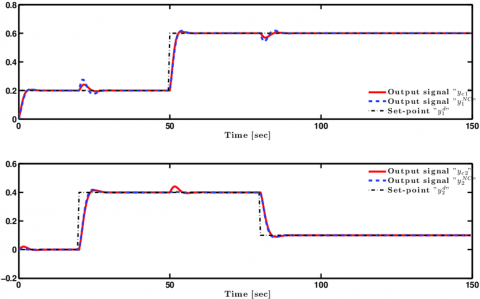
Figure 5. Evolution versus time of the output responses of Tank 1 and Tank 3, obtained with classical C-MPC and the proposed NC-DMPC for the quadruple tank system

6.png

Figure 6. Evolution versus time of the manipulated variables (control inputs); $v_1$ and $v_2$; generated by classical C-MPC and the proposed NC-DMPC schemes for the control of the quadruple tank system

7.png

Figure 7. Evolution versus time of the output responses of Tank 1 and Tank 3, obtained with decentralized MPC and the proposed NC-DMPC for the quadruple tank system

8.png

Figure 8. Evolution versus time of the manipulated variables (control inputs); $v_1$ and $v_2$; generated by decentralized MPC and the proposed NC-DMPC schemes for the control of the quadruple tank system

Table 1. Summary of the control design parameters of the different MPC controllers

Note that the design parameters N_p, R_i, Q_i, p_i and $\mathcal{N}_i$, for i=1,2 needed for the distributed optimization problem, have been manually (i.e., heuristically) tuned to obtain the best performance. To this end, several tests were performed to determine the most suitable values for the proposed case. Besides, the optimal values can be found using a multi-objective optimization procedure or one of the metaheuristic methods (such as swarm optimization technique), but this is out of the scope of this study. Usually, a trade-off between the two terms of the performance index should be ensured, depending on each particular circumstance (response rapidity or lower energy).

In order to make a fair comparison, the closed-loop performance of the proposed controller are compared with a Laguerre functions-based Decentralized MPC (DeMPC), where the network communication is omitted (Figure 1(b)), and a classical centralized MPC (C-MPC). The simulation parameter settings are summarized in Table 1.

where, N_u denotes the control horizon, it is selected by considering a good trade-off between tracking performance and the amount of the control effort; N_p is the prediction horizon, it is assumed sufficiently large, to ensure the closed-loop stability. Q and R are two constant matrices serving as weights of the tracking errors and control actions, respectively; p_i is the scaling factor, it is a tuning parameter for the closed-loop response speed; $\mathcal{N}_i$ is the number of Laguerre functions representing the degrees of freedom in describing the control trajectory; T_s is the sampling time; N^s is the total number of samples of the whole simulation.

For this example, the obtained simulation results are depicted in Figures 5, 6, 7 and 8, including the system outputs and the generated control signals. The obtained simulation results, demonstrate that the proposed distributed control structure has a good control performance, since the quadruple tank system under the proposed DMPC strategy has the ability to track the set-point signals; with smooth control signals. Although, the control signals in this control strategy are obtained separately, the performance is still satisfactory due to the cooperative manner of the sub-controllers by using the local information and the information shared by the other agents via the communication network.

Furthermore, as depicted in Figures 5 and 6, the C-MPC has a similar performance as the proposed NC-DMPC, and both outperform the DeMPC strategy, as shown in Figures 7 and 8. This conclusion is not only valid for this four tank plant, but also for other plants, since the DeMPC strategies does not take the interactions into account, which leads to some degradation in performance. It is noteworthy to mention that the main drawback of decentralized MPC is that local MPC controllers would fail to fully compensate for the process interactions beyond the confines of the local subsystems. Such limitation can degrade the controller performance and possibly, leads to stability problems of the overall system.

The computational burden of the control schemes depends greatly on the number of inequality constraints and the number of control variables [51]. From this point of view, in the unconstrained centralized MPC, the optimization problem increases significantly with the total number $\mathbf{u}^{\{i\}}$ of system inputs as well as the length of the control horizon $N_u$, since a large value of the control horizon implies more control variables to be computed. In the proposed NC-DMPC strategy, the local control actions are parameterized by Laguerre functions. The total number of Laguerre functions, namely $\mathcal{N}$, used in capturing the future control trajectory vector is generally less than $N_u$. Thereby, each sub-controller needs smaller control variables to be computed, compared to the classical centralized control scheme.

Incidentally, by decomposing the problem into smaller subproblems and solving them in parallel, we can handle a much larger number of units. Furthermore, compared to the classical centralized algorithms, decomposition methods require less memory storage, and are mainly much faster. To sum up, the computational burden of the distributed implementation is much less than the centralized structure, especially for large-scale systems including a large number of subsystems.

8.2 Performance analysis discussion

The performance analysis of the control strategies can be described in terms of output tracking errors and control efforts. Therefore, a more accurate way to obtain a criterion reflecting the performance and differences between the different MPC controllers is to evaluate the following unified performance index,

$J_{i(k)}=\sum_{k=1}^{N^s}\left\|\hat{\mathrm{y}}_{(k)}^{\{i\}}-\mathrm{y}_{(k)}^{\{i\} s p}\right\|_{Q_i}^2+\sum_{k=1}^{N^s}\left\|\Delta \mathrm{u}_{(k)}^{\{i\}}\right\|_{R_i}^2=\sum_{k=1}^{N^s} J_{e_i(k)}+\sum_{k=1}^{N^s} J_{u_i(k)}$ for $i=1,2$.    (45)  

where, $N^s$ represents the total number of samples of the whole simulation, $\mathrm{y}^{\{i\} s p}$ denotes the set-point (reference) to be tracked and $\mathrm{y}^{\{i\}}$ is the actual simulated output. The MPC performance index in (45) is formulated with two performance indices, namely the tracking error and the control effort. The performance index corresponding to the tracking error $J_{e_i}$ is formulated using the squared difference between the set-point $y^{s p}$ and the predicted plant behavior $\hat{y}$. Similar to the tracking error term, the performance index for the control effort $J_{u_i}$ is also formulated as in (45). The control effort is determined by the squared difference between the present and past control actions.

It is worth to recall that one key concept in centralized control is that all the individual performance indices J_i are gathered in a single cost function, leading to:

$J_{(k)}^{\text {cost }}=\sum_{i=1}^{\mathbb{N}=2} J_{i(k)}=\sum_{i=1}^{\mathbb{N}=2}\left(\sum_{k=1}^{N^s} J_{e_i(k)}+\sum_{k=1}^{N^s} J_{u_i(k)}\right)$     (46a)

$=\sum_{i=1}^{\mathbb{N}=2} \sum_{k=1}^{N^s} J_{e_i(k)}+\sum_{i=1}^{\mathbb{N}=2} \sum_{k=1}^{N^s} J_{u_i(k)}$      (46b)

$J_{(k)}^{\cos t}=J_{e(k)}+J_{u(k)}$      (46c)

The evaluation results are summarized in Table 2.

Table 2. Comparison of the costs obtained with centralized MPC, distributed MPC and decentralized MPC

Table 2 shows the results obtained through the evaluation of the performance index (46) for the three MPC controllers. As it can be seen from this table, the same previous conclusion holds according to the obtained numerical values. It shows that decentralized MPC has the largest value of the global performance index $J^{cost}$, whereas the proposed distributed NC-MPC has a performance close to the centralized scheme. Taking into account each term of the performance index, the proposed DMPC has almost the same performance compared to the C-MPC controller; and both have a better performance related to the tracking error, but the De-MPC and C-MPC controllers have a slightly smaller control efforts compared to the proposed DMPC. Using the proposed NC-DMPC scheme, the tank levels track the set-point signals better than with the controller De-MPC. This is because the distributed MPC controller provides more control effort than decentralized MPC scheme. The obtained results of the above table, with Figures 7 and 8, corroborate this conclusion.