Suha S. Husain* | Taghreed MohammadRidha
© 2022 IIETA. This article is published by IIETA and is licensed under the CC BY 4.0 license (http://creativecommons.org/licenses/by/4.0/).
OPEN ACCESS
Seismic effects control in recent years has attracted considerable attention to reduce their effects for the safety of humans and structures. Therefore, in this work Integral Sliding Mode Control Based on Barrier Function (ISMCbf) is applied for the first time to regulate the displacement of a three-story scaled structure against earthquake excitation. This new type of controller does not need any information of the upper bound of the disturbance. Firstly, the controller is applied to a semi active Magneto Rheological Damper (MRD) and compared to the performance of Active Tuned Mass Damper (ATMD) under the effect of two different simulated earthquakes: time scaled El Centro 1940 earthquake and Mexico City earthquake. ISMCbf with MRD reduced the displacement of the structure with lower required controlled force as compared to ATMD with ISMCbf behavior. Secondly, the efficiency of ISMCbf with MRD is shown when compared to other controllers with MRD from previous studies.
active control, semi active control, ATMD, MRD, seismic effect, integral sliding mode, integral sliding mode control with barrier function, earthquake vibration
The reduction of vibrations in structures resulting from seismic effects is the primary objective of engineers in this field. Seismic effects have impacts on people and structures, and many of these structures are very effective in serving people, they should remain functional even after earthquakes. For this purpose, several techniques have been proposed to minimize the seismic impact.
All these devices and seismic control methods have benefits and flaws. One type of these devices is the passive control, which depends on energy dissipation and has no external energy source. Passive control principle is to isolate the building from the ground by means of energy dissipation devices such as Tuned Mass Damper (TMD) [1]. It doesn't have a feedback correction signal of a controller, so it is not sufficient to control external perturbations [2]. Therefore, active control dampers were designed which operate on an external power source directed by a control algorithm. The control signal is generated by a control algorithm that used feedback measurements of the state variables of the structure [3].
Active control dampers like Active Tuned Mass Damper (ATMD), are efficient but has the drawback of requiring a high power source [4]. As a result, semi-active control has emerged, which require low power supply to work, like Magneto Rheological Damper (MRD) [5]. Semi active control is a combination of passive control and active control. Its active portion is only used when there is high building excitation, otherwise, it behaves passively. The force of these devices is adjustable based on the control of fluid viscosity using electrical or magnetic fields supplied by low-power batteries [6].
The objective of many studies in this field was to design a suitable robust control algorithm for active and also semi active dampers. Some researchers designed classical controllers, others designed intelligent control. Kavyashree and Rao [7] proposed proportional–integral–derivative (PID) controller with MRD to control a scaled structure to reduce earthquake effect. The controller was checked under three types of earthquakes. While Zizouni et al. [8] they designed Linear Quadratic Regulator (LQR) to control a scaled structure with MRD. In the two previous studies researchers used classical control for the purpose of reducing seismic effect. As is known, classical control is insufficient to control the systems that is exposed to external disturbances. Yan et al. [9] proposed Fuzzy Neural Network algorithm (FNN) and compared it with LQR to control a symmetric building with ATMD on the top floor, they concluded that FNN performance was better than LQR. However, FNN needs training in design and requires prior knowledge of the perturbations upper bound. Concha et al. [10] designed Sliding Mode Control (SMC) to control a scaled structure with ATMD and compared its performance with the traditional LQR, they checked the two designs under effect of time scaled El Centro 1940 earthquake, they concluded that SMC was better than LQR performance. This study used ATMD as actuator which needs high power supply. Khatibinia et al. [11] proposed Optimal Sliding Mode Control (OSMC) to control 11- story building with ATMD in the top floor, the proposed controller compared to PID, LQR and fuzzy logic controller, the concluded OSMC has the better performance than other controllers. Humaidi et al. [12] and Fali et al. [13] the authors designed Adaptive Sliding Mode Control (ASMC) with MRD to control a scaled structure. They compared ASMC with SMC response to show the efficiency of the former. In the previous studies SMC, ASMC and OSMC required the prior knowledge of disturbance upper bounds.
In summary highlighted from the robust controllers in previous studies that SMC, ASMC and OSMC all these controllers need the upper bound of the disturbance in its design. Moreover, these robust controllers have discontinuous term that causes chattering phenomenon which means these controllers need some kind of approximation to attenuate it.
From the previous drawbacks, the motivated that lead to overcomes this problem by Husain and Ridha [14] to design Integral Sliding Mode Based on barrier function (ISMCbf). They compared three types of controllers: SMC, Integral Sliding Mode Controller (ISMC) and ISMCbf to control the behavior of ATMD placed on the top floor of a scaled structure. The results showed that SMC, ISMC and ISMCbf succeeded in reducing the maximum displacement, but ISMCbf reduced the applied force by 52 percent i.e. it reduced the required energy. The most important advantage in designing this new proposed controller (ISMCbf) is that it does not require the upper bounds of the external disturbance nor the uncertainties in it design [15]. As mention earlier ATMD needs high power supply and high cost. Moreover, it’s difficult maintain, and there are constraints in its performance. Therefore, in this study ISMCbf is designed for the first time to control MRD to reduce seismic structural vibrations and also minimizing the required control energy. ISMCbf has shown to be simple in design and does not need prior knowledge of the perturbations upper bound. Moreover, this controller is not discontinuous, therefore it is not needing any kind of approximation to avoid chattering. This new control strategy is compared to the results of ISMCbf with ATMD under two different simulated earthquakes. Both dampers were placed on the top floor of a three-story scaled structure. To show the efficiency of ISMCbf control algorithm, the performance of ISMCbf with MRD is compared to other control algorithms from the literature [16-18] which used the same MRD for the same scaled structure. ISMCbf algorithm has proven its efficiency in reducing both the displacement and also reducing the control force compared to other control algorithms.
This paper is organized as follows: The mathematical model of a building with ATMD and MRD is presented in section 2. Integral sliding mode control design is explained in section 3. In section 4, the results are presented and discussed. Finally, the conclusion is presented in section 5.
The mathematical model of a building is shown in Eq. (1) [10]:
$M \ddot{x}(t)+C \dot{x}(t)+K x(t)=M \Lambda \ddot{x}_g(t)-\Gamma F_c(t)$ (1)
where, $x, \dot{x}$ and $\ddot{x}$ are displacement, velocity and acceleration vectors of the structure respectively, where $\boldsymbol{x}$ is the displacement vector which represented as $x=$ $\left[x_1, x_2, x_3, \ldots, x_n\right]^T, n$ is the number of floors and in this work $\boldsymbol{n}=3$. C, $K$ and $M \in R^{n * n}$ are damping, stiffness and mass matrices. $M$ is a diagonal matrix. $C$ and $K$ are tridiagonal matrices. $\ddot{x}_g$ is the earthquake acceleration. $\Lambda \epsilon R^{n * 1}$ is unity vector, $F_c$ is the force produced by the dampers, $\Gamma \in R^{n * 1}$ represent the location of each damper. In this work one damper will be considered, hence:
$\boldsymbol{\Gamma}=[0,0,0,0,0,1]^T$ (2)
State space representation for (1) is as follows:
$\dot{\boldsymbol{x}}=\boldsymbol{A} \boldsymbol{x}+\boldsymbol{B} u+\boldsymbol{D} \ddot{x}_g$ (3)
where, $\boldsymbol{B}$ and $\boldsymbol{D}$ are $\epsilon R^{2 n * 1}, \boldsymbol{A} \in R^{2 n * 2 n}, u=F_c$. These matrices are as flows:
$A=\left[\begin{array}{cc}0 & I \\ -M^{-1} K & -M^{-1} C\end{array}\right], B=\left[\begin{array}{c}0 \\ -M^{-1} \Gamma\end{array}\right], D=-\left[\begin{array}{l}0 \\ \Lambda\end{array}\right]$.
2.1 Mathematical model of ATMD
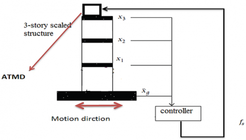
ATMD is placed on the top floor of the three-floor scaled structure as shown in Figure 1. The principle of ATMD is to produce forces that are opposite to the seismic forces [11].
Figure 1. Shows ATMD on the top floor
The following equations represent the mathematical model of ATMD [10]:
$m_d\left(\ddot{x}_d(t)+\ddot{x}_n(t)+\ddot{x}_g(t)\right)=F_c(t)$ (4)
$F_c(t)=f_s-k_d x_d(t)-c_d \dot{x}_d(t)$ (5)
where, $m_d, k_d, c_d$ are mass, stiffness, and damping of ATMD respectively. $f_s$ is the control signal applied to the ATMD, $F_c(t)$ is the net force acting upon the ATMD. $\ddot{x}_n(t)$ is the acceleration of the top floor.
2.2 Mathematical model of MRD
MRD shown in Figure 2 is one of the most important semi-active dampers. MRD consists of a hydraulic cylinder, which is separated using a piston head. The cylinder is filled with a special properties fluid (viscous fluid), which can pass through the small orifices. The two sides of cylinder are connected using an external valve which is used to control the device operation. The semi-active stiffness control device modifies the system dynamics by changing the structural stiffness [12]. Moreover, it is powered by a small battery because it needs less than 50 Watt of power also, MRD response in milliseconds and operate with temperature range -40℃ to + 150℃ [12]. MRD is preferred for seismic control because it is easy to install and maintain and it can be placed on any floor of the building because of its small size. The model of MRD is nonlinear which is described by the modified Bouc–Wen model, this model was proposed by Yu and Thenozhi [19] as follows:
$F_c=c_1 \dot{y}+k_0(x-y)+k_1\left(x-x_o\right)+\alpha z$ (6)
$\dot{y}=\frac{1}{c_0+c_1}\left(c_o \dot{x}+k_o(x-y)+\alpha z\right)$ (7)
$\dot{z}=-\gamma|\dot{x}-\dot{y}| z|z|^{r-1}-\beta(\dot{x}-\dot{y})|z|^r+a(\dot{x}-\dot{y})$ (8)
where, $x$ and $\dot{x}$, are displacement and velocity of the damper respectively, $F_c, z, k_o$ and $k_1$ are generated force, hysteretic component, accumulator stiffness respectively at low and high velocity. $\Upsilon, \beta, r$ and $a$ are parameters giving the shape and scale of the hysteresis loop. $c_o$ and $c_1$ are the viscous damping at low and high velocity respectively, which depend on control voltage as see in Eqns. (9), (10), (11) and (12) respectively:
$\alpha=\alpha_a+\alpha_b \mu$ (9)
$c_1=c_{1 a}+c_{1 b} \mu$ (10)
$c_o=c_{o a}+c_{o b} \mu$ (11)
$\dot{\mu}=-\eta\left(\mu-v_c\right)$ (12)
where, $\eta$ is time response factor, $\mu$ is a phenomenological variable enveloping the system and vc is the command voltage applied to the control circuit of the damper.
Figure 2. Schematic representation of an MR damper implemented in a three-story building
The resulting supplied control voltage of MRD is as follows [8, 16, 17]:
$v_c=v_{\max } H\left\lceil\left(f_s-F_c\right) \cdot F_c\right]$ (13)
where, vmax is maximum applied voltage, fs the output force of controller (control force) and Fc force generated by MRD. H(.) is a Heaviside step function.
SMC is a robust control, which deals with matched disturbances and uncertainties. SMC is widely used due to its preferred robust performance [10, 20, 21]. SMC has two phases, reaching phase and sliding phase. In reaching phase, the controller will derive state will trajectory toward the sliding manifold in-finite time. In sliding phase when the state trajectory gets on the sliding manifold, the trajectory will remain on this manifold, and then it moves along the sliding manifold until it reaches the origin asymptotically. During reaching phase the system is affected by external disturbances, while during sliding phase the system is not affected by external disturbances [22, 23]. Therefore, it is desired to reduce the reaching phase. ISMC eliminates the reaching phase in it is design [22]. Both SMC and ISMC need the upper bound of disturbance in the design procedure. A new ISMCbf is recently designed such that it does not require any prior knowledge of the perturbations bounds [23, 24]. This new control algorithm has the following advantages [15, 25]:
The strategy does not require any prior knowledge of the perturbations bounds.
Simpler in design, where its design needs one parameter to be specified only that defines the steady-state error accuracy.
The algorithm is a smooth function, so it does not need any approximation to avoid chattering effect caused by the conventional discontinuous of ISMC.
ISMCbf is designed for the system in Eq. (3) with $A \in$ $R^{6 * 6}$, and $\boldsymbol{D}, \boldsymbol{B} \in R^{6 * 1}$. Firstly, the barrier function will be defined as follows:
Definition [15, 25, 26]: For some given fixed ε>0; the barrier function can be defined as even continuous function $\mathrm{f}: \mathrm{x} \in[-\varepsilon, \varepsilon] \rightarrow \mathrm{g}(\mathrm{x}) \in[\mathrm{b}, \infty]$ strictly increasing on [0, $\mathcal{E}$].
$\lim _{|x|} \rightarrow \varepsilon g(x)=+\infty$
g(x) has a unique minimum at zero and g(0)= b$\geq$0
there are two different classes of Barrier Functions (BFs) as follows:
1. Positive definite BFs (PBFs):
$g_p(x)=\frac{\varepsilon F}{\varepsilon-|x|}, g_p(0)=F>0$ (14)
2. Positive Semi-definite BFs (PSBFs):
$g_{p s}(x)=\frac{|x|}{\varepsilon-|x|}, g_{p s}(0)=0$ (15)
The $g_{p s}(x)$ is used in this work. The first step in the design procedure is to design the sliding surface:
$\sigma=G x+Z$ (16)
where, $\sigma$ is the sliding manifold, $Z$ is the integral term, $G \in \mathrm{R}^{1 * 6}$ to be designed. The derivative of sliding manifold and the integral term which
$\dot{\sigma}=G \dot{x}+\dot{Z}$ (17)
$\dot{Z}=-G A \, x-u_n$ (18)
Finally, ISMCbf control action produced in Eq. (19);
$u=(G B)^{-1}\left(u_n+u_d\right)$ (19)
where, un and ud are the nominal controller and discontinuous controller respectively which are designed as follows:
$u_n=-K_1 x$ (20)
$u_d=-\frac{\sigma}{\epsilon-|\sigma|}$ (21)
where, $K_1$ is the gain vector designed using Ackermann’s formula, $\epsilon$ is very small positive constant.
After substituting Eq. (19) in Eq. (3) then Eqns. (18) and (3) in Eq. (17) the result as follows:
$\dot{\sigma}=u_d+G D \ddot{x}_g$ (22)
To write the system dynamics during sliding ( $\dot{\sigma}=0$ ), the equivalent control is:
$[\dot{\sigma}]_{e q}=0=\left[u_d\right]_{e q}+G D \ddot{x}_g$ (23)
$\left[u_d\right]_{e q}=-G D \ddot{x}_g$ (24)
Substituting in Eq. (3), the resulting system dynamics is described as follows:
$\dot{x}=\left(A-B K_1\right) x$ (25)
The above system is stable by choosing $K_1$ matrix to be Hurwitz. To ensure attractiveness of sliding surface $\sigma$ the condition below must be satisfied [27];
$\sigma \dot{\sigma}<0$ (26)
After substituting Eq. (21) in (22) then in (26) the result is;
$\sigma \dot{\sigma}=\sigma\left(-\frac{\sigma}{\epsilon-|\sigma|}+G D \ddot{x}_g\right)<0$ (27)
Let $G D \ddot{x}_g=\delta$ is assumed bounded with unknown upper bound $|\delta|$, taking the bounds of (27):
$\sigma \dot{\sigma} \leq-|\sigma|\left(\frac{|\sigma|}{|\epsilon-| \sigma||}-|\delta|\right)$ (28)
Therefore $\sigma \dot{\sigma}<0$ for $|\sigma|$ sufficiently near $\epsilon$ where $\frac{|\sigma|}{|\epsilon-| \sigma||}>|\delta|$. Therefore, the set $\Omega=\{x:|\sigma| \leq \epsilon\}$ is positively invariant.
ISMCbf drives the system to start inside the small neighborhood of |σ|<ϵ; and as this set is invariant. Therefore, the controller rejects the disturbance from the first instance. The preferred robustness of ISMC is improved by adding the barrier function where with ISMCbf the upper bound of the system perturbations are not required [15, 25]. Only one control parameter is to be chosen $\epsilon$, which is very small positive constant that defines the barrier function invariant set.
In this section a three-floor scaled structure is taken as a case study whose parameters are presented in Table 1. All initial conditions are set to zero (starting from rest). The simulations results presented below were categorized into two scenarios: firstly, the responses of using ATMD and MRD both controlled by ISMCbf are compared under time scaled Mexico City earthquake and time scaled El Centro 1940 earthquake. The purpose of this scenario is to show the performance differences between ATMD and MRD under the same control algorithm. The objective of the second scenario is to show the efficiency of ISMCbf control algorithm with the MRD as compared to other controllers which employed the same MRD from the literature [16, 17].
4.1 Scenario I: ATMD versus MRD comparison
The three-story scaled structure which parameter is given in Table 1 [16]. ATMD and MRD are both controlled by ISMCBF and are placed on the top floor thus G=G1=[0,0,0,0,0,1]. The structure is exposed to two different earthquakes: time scaled Mexico City earthquake and time scaled El Centro 1940 earthquake. The parameters of these dampers are given in Table 2 [16, 28]. The control parameters are shown in Table 3.
Table 1. System parameter
|
Parameter name |
Parameter value |
|
Mass matrix (M) Kg |
$\left[\begin{array}{ccc}98.3 & 0 & 0 \\ 0 & 98.8 & 0 \\ 0 & 0 & 98.3\end{array}\right]$ |
|
Damping matrix (C)N.s/m |
$\left[\begin{array}{ccc}175 & -50 & 0 \\ -50 & 100 & -50 \\ 0 & -50 & 50\end{array}\right]$ |
|
Stiffness matrix (K) N/m |
$10^5 \times\left[\begin{array}{ccc}12 & -6.84 & 0 \\ -6.84 & 13.7 & -6.84 \\ 0 & -6.84 & 6.84\end{array}\right]$ |
Table 2. Actuators parameters
|
MRD parameters. |
Parameter name |
Parameter value |
|
$C_{0 a}, C_{0 b}$ |
$21,3.5^{\mathrm{N} \cdot \mathrm{s}} / \mathrm{cm}$ |
|
|
$k_0, a$ |
46.9 N/cm, 301 |
|
|
$c_{1 a}, c_{1 b}$ |
$283 \mathrm{~N} . \mathrm{s} / \mathrm{cm} 2.95 \mathrm{~N} \cdot \mathrm{s} / \mathrm{cm}$ |
|
|
r |
2 |
|
|
$\alpha_a, \alpha_b$ |
$140 \frac{\mathrm{N}}{\mathrm{cm}}, 695 \mathrm{~N} / \mathrm{cm}$ |
|
|
$\gamma, \beta$ |
$363 \mathrm{~cm}^{-2}, 363 \mathrm{~cm}^{-2}$ |
|
|
$\eta, x_0$ |
$190 \mathrm{~s}^{-1}, 14.3 \mathrm{~cm}$ |
|
|
$\nu_{\max }$ |
$2.25 v$ |
|
|
ATMD parameters. |
$m_d$ |
$2.89 \mathrm{~kg}$ |
|
$C_d$ |
$2.37 \times 10^{-3} N s / m$ |
|
|
$k_d$ |
$3.84 \times 10^3 N / m$ |
Table 3. Controllers parameters
|
Parameter name |
Parameter value |
|
$G_1$ |
$\left[\begin{array}{llllll}0 & 0 & 0 & 0 & 0 & 1\end{array}\right]$ |
|
$G_2$ |
$\left[\begin{array}{llllll}0 & 0 & 0 & 1 & 0 & 0\end{array}\right]$ |
|
$\epsilon$ |
0.0001 |
Figure 3. Scaled acceleration of Mexico City earthquake
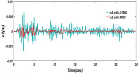
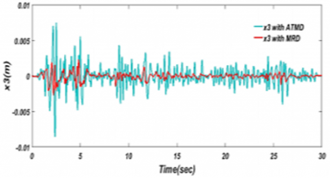
Displacement of the three stories under effect of Mexico City earthquake controlled by ISMCbf with using ATMD and MRD. The results are shown in Figure 5. From the results clear that it is ISMCbf with MRD is better than ISMCbf with ATMD in reducing both displacement and control force [29].
(a) First floor displacement
(b) Second floor displacement
(c) Third floor displacement
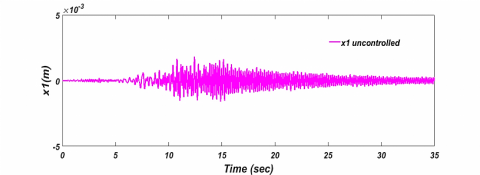
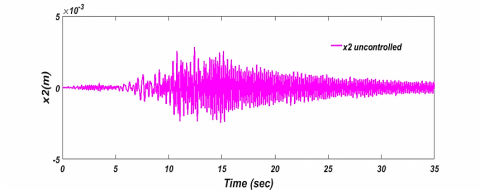
Figure 4. Uncontrolled Displacement of three floors under effect of scaled Mexico City Earthquake
(a) First floor displacement
(b) Second floor displacement
(c) Third floor displacement
Figure 5. Displacement for three floors under effect of Mexico City earthquake with ATMD and MRD controlled by ISMCbf
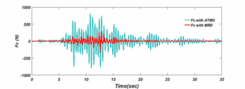
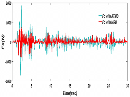
Figure 6. The control force by ATMD and MRD under effect of time scaled Mexico City earthquake
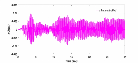
The uncontrolled displacements of the three floors are illustrated under time scale Mexico City earthquake in Figures 3 and 4 respectively.
The control forces Fc produced by ATMD and MRD are shown in Figure 6.
The statistical results of the compared actuators results controlled by ISMCbf under effect of Mexico City earthquake are given in Table 4.
Time scaled El Centro 1940 earthquake is also applied to test the controlled system. The results shown in Figure 7 illustrates the open-loop response for three stories. Moreover, the displacements of the three stories under effect of time history El Centro 1940 earthquake controlled by ISMCbf with using ATMD and MRD are shown in Figure 8.
The control forces Fc produced by ATMD and MRD are shown in Figure 9 under effect of time scaled El Centro 1940 earthquake.
Table 4. Maximum structural responses when structure is subjected to the Mexico City earthquake using ATMD and MRD
|
|
Uncontrolled |
ISMCbf |
|
|
ATMD |
MRD |
||
|
1st floor displacement (m) |
0.002 |
0.00148 |
0.0003 |
|
2nd floor displacement (m) |
0.003 |
0.00235 |
0.00046 |
|
3rd floor displacement (m) |
0.0034 |
0.0029 |
0.000548 |
|
Control force(N) (Fc) |
/ |
810 |
300 |
(a) First floor displacement
(b) Second floor displacement
(c) Third floor displacement
Figure 7. Uncontrolled displacement for three floors under effect of El Centro 1940 earthquake
Table 5. Maximum structural responses under time scaled El Centro 1940 earthquake
|
|
Uncontrolled |
ISMCbf |
|
|
ATMD |
MRD |
||
|
1st floor displacement(m) |
0.0055 |
0.0042 |
0.00127 |
|
2nd floor displacement(m) |
0.0083 |
0.0064 |
0.00197 |
|
3rd floor displacement(m) |
0.0097 |
0.074 |
0.00233 |
|
Control force(N) $\left(F_c\right)$ |
/ |
1859.8 |
751 |
The statistical results of the compared actuators results controlled by ISMCbf under effect of time scaled El Centro 1940 earthquake are given in Table 5.
The results show that MRD performance in reducing displacement caused by earthquake effect dominated that of the ATMD with less control force Fc as can be seen in Tables 4 and 5.
(a) First floor displacement
(b) Second floor displacement
(c) Third floor displacement
Figure 8. Displacement for three floors under effect of El Centro 1940 earthquake with ATMD and MRD controlled by ISMCbf
Figure 9. The control force by ATMD and MRD under effect of time scaled El Centro 1940 earthquake
4.2 Scenario II: ISMCbf comparison with other controllers
To show the efficiency of ISMCbf control algorithm with the MRD, it will be compared to other controllers from the literature [16, 17] which used the same MRD and same structure. The three-floor system parameters are shown in Table 1. The MRD is placed on the ground floor, therefore G=G2=[0,0,0,1,0,0] as given in Table 3.
The statistical results of the proposed controller under effect of El Centro 1940 earthquake are given in Table 6.
From the comparison with the results were obtained by [16, 17], show that proposed control technique is better in terms of control force than all control techniques except those proposed control algorithms No.2 and 8 respectively, but when compare the displacement which obtained by ISMCbf, ISMCbf result is better than the above two algorithms as well as from all technics which proposed by Aly et al. [16, 17]. In addition to all of the above, this type of control algorithm does not need any information about the upper bound disturbance.
Table 6. Comparison of maximum structural responses between ISMCbf performance and the proposed controllers [16, 17]
|
|
Control strategy |
$x_3$ (m) |
$F_c$ (N) |
|
1 |
Uncontrolled |
0.0055 0.0083 0.0097 |
/ |
|
2 |
Passive off |
0.0021 0.0036 0.0045 |
259.2 |
|
3 |
Passive on |
0.0008 0.002 0.0031 |
992.8 |
|
4 |
Lyapunov controller (A) |
0.0009 0.0021 0.0031 |
1023 |
|
5 |
Lyapunov controller (B) |
0.0013 0.0018 0.0023 |
993.3 |
|
6 |
Quasi-bang-bang controller |
0.0013 0.0016 0.0023 |
1002 |
|
7 |
Decentralized bang-bang controller |
0.0015 0.0025 0.0032 |
923 |
|
8 |
Modulated homogenous friction controller |
0.0019 0.0029 0.0038 |
503 |
|
9 |
Maximum energy dissipation controller |
0.0008 0.0020 0.0031 |
993 |
|
10 |
Clipped-optimal controller |
0.0014 0.0021 0.0026 |
918 |
|
11 |
Modified Quasi-bang-bang controller |
0.0012 0.0019 0.0027 |
848.9 |
|
12 |
ISMCbf |
0.00086 0.00136 0.00144 |
704.4 |
In this work ISMCbf is designed for the first time to drive MRD to regulate structural vibrations under earthquakes. This new control strategy has the preferred robustness of ISMC and more importantly has the barrier invariant set the confines the state trajectory within rejecting the external perturbations. The barrier function ISMC is designed without prior knowledge of any disturbance upper bounds. ISMCbf can reject the disturbances by defining the barrier function parameter only. ISMCbf is tested in two scenarios. In the first simulation scenario ISMCbf with MRD is compared to ISMCbf with ATMD under two different earthquakes of unknown bounds. It was shown that MRD performance is better than ATMD in mitigating structural vibrations. ISMCbf with MRD reduced structural displacement with less required control energy as compared to ISMCbf with ATMD. In the second scenario, ISMCbf with MRD is compared to other control strategies from the literature which employed the same MRD on the same scaled structure. ISMCbf performance was better than most of the other control strategies in reducing both the control signal and the structural vibrations. The following points resumes the main concluding remarks:
ISMCbf with MRD can reduce the displacement better than ATMD with less control force Fc, and it is derived by small battery level voltage (0-2.25V). As a result, MRD more reliable than ATMD during sever earthquakes.
ISMCbf is preferred due to its robustness and simple design as does not require any information of upper bound of disturbance. Its comparison with other control strategies in this work proved its efficiency in reducing structural vibrations.
ISMCbf is smooth continuous controller, which does not require any sort of filtration or approximation to avoid chattering due to the discontinuous control term that is found in conventional SMC and ISMC.
As a future work a practical implementation may be proposed on a scaled structure and MRD prototype to validate the simulation results, then study if there any problems before applied the design on the real buildings.
[1] Ridha, T.M.M. (2010). The design of a tuned mass damper as a vibration absorber. Engineering and Technology Journal, 28(14): 4844-4852
[2] Mahmoud, U.Y., Yasien, F.R., Ridha, T.M.M. (2009). Sliding mode control for gust responses in tall building. Engineering and Technology Journal, 27(5): 983-992.
[3] Ulusoy, S., Nigdeli, S.M., Bekdaş, G. (2021). Novel metaheuristic-based tuning of PID controllers for seismic structures and verification of robustness. Journal of Building Engineering, 33: 101647. https://doi.org/10.1016/j.jobe.2020.101647
[4] Owji, H.R., Shirazi, A.H.N., Sarvestani, H.H. (2011). A comparison between a new semi-active tuned mass damper and an active tuned mass damper. Procedia Engineering, 14: 2779-2787. https://doi.org/10.1016/j.proeng.2011.07.350
[5] Ikeda, Y., Sasaki, K., Sakamoto, M., Kobori, T. (2001). Active mass driver system as the first application of active structural control. Earthquake Engineering & Structural Dynamics, 30(11): 1575-1595. https://doi.org/10.1002/eqe.82
[6] Kotla, R.W., Yarlagadda, S.R. (2020). Grid tied solar photovoltaic power plants with constant power injection maximum power point tracking algorithm. Journal Européen des Systèmes Automatisés, 53(4): 567-573. https://doi.org/10.18280/jesa.530416
[7] Kavyashree, Jagadisha, H.M., Rao, V.S., Bhagyashree (2020). Classical PID controller for semi-active vibration control of seismically excited structure using magneto-rheological damper. In: Sivasubramanian, V., Subramanian, S. (eds) Global Challenges in Energy and Environment. Lecture Notes on Multidisciplinary Industrial Engineering. Springer, Singapore. https://doi.org/10.1007/978-981-13-9213-9_19
[8] Zizouni, K., Bousserhane, I.K., Hamouine, A., Fali, L. (2017). MR Damper-LQR control for earthquake vibration mitigation. International Journal of Civil Engineering and Technology (IJCIET), 8(11): 201-207.
[9] Yan, X., Xu, Z.D., Shi, Q.X. (2020). Fuzzy neural network control algorithm for asymmetric building structure with active tuned mass damper. Journal of Vibration and Control, 26(21-22): 2037-2049. https://doi.org/10.1177/1077546320910003
[10] Concha, A., Thenozhi, S., Betancourt, R.J., Gadi, S.K. (2021). A tuning algorithm for a sliding mode controller of buildings with ATMD. Mechanical Systems and Signal Processing, 154: 107539. https://doi.org/10.1016/j.ymssp.2020.107539
[11] Khatibinia, M., Mahmoudi, M., Eliasi, H. (2020). Optimal sliding mode control for seismic control of buildings equipped with ATMD. Iran University of Science & Technology, 10(1): 1-15.
[12] Humaidi, A.J., Sadiq, M.E., Abdulkareem, A.I., Ibraheem, I.K., Azar, A.T. (2021). Adaptive backstepping sliding mode control design for vibration suppression of earth-quaked building supported by magneto-rheological damper. Journal of Low Frequency Noise, Vibration and Active Control, 41(2). https://doi.org/10.1177/14613484211064659
[13] Fali, L., Djermane, M., Zizouni, K., Sadek, Y. (2019). Adaptive sliding mode vibrations control for civil engineering earthquake excited structures. International Journal of Dynamics and Control, 7(3): 955-965. https://doi.org/10.1007/s40435-019-00559-0
[14] Husain, S.S., MohammadRidha, T. (2022). Design of integral sliding mode control for seismic effect regulation on buildings with unmatched disturbance. Mathematical Modelling of Engineering Problems, 9(4): 1123-1130. https://doi.org/10.18280/mmep.090431
[15] Abd, A.F., Al-Samarraie, A.S. (2021). Integral sliding mode control based on barrier function for servo actuator with friction. Engineering and Technology Journal, 39(2): 248-259. https://doi.org/10.30684/etj.v39i2A.1826
[16] Aly, A.M. (2013). Vibration control of buildings using magnetorheological damper: a new control algorithm. Journal of Engineering, 2013. https://doi.org/10.1155/2013/596078
[17] Dyke, S.J., Spencer, B.F. (1997). A comparison of semi-active control strategies for the MR damper. In Proceedings Intelligent Information Systems. IIS'97, pp. 580-584. https://doi.org/10.1109/IIS.1997.645424
[18] Kayabekir, A.E., Bekdaş, G., Nigdeli, S.M., Geem, Z.W. (2020). Optimum design of PID controlled active tuned mass damper via modified harmony search. Applied Sciences, 10(8): 2976. https://doi.org/10.3390/app10082976
[19] Yu, W., Thenozhi, S. (2016). Active structural control with stable fuzzy PID techniques. Springer International Publishing. https://doi.org/10.1007/978-3-319-28025-7
[20] Abd, A.F. (2021). Sliding mode controller for motor-quick-return servo mechanism. A M. Sc. Thesis Presented to the Control and Systems Eng. Dept., University of Technology, Baghdad, Iraq.
[21] Rakan, A.B., Mohammad, T., AL-Samarraie, S.A. (2022). Artificial pancreas: Avoiding hyperglycemia and hypoglycemia for type one diabetes. International Journal on Advanced Science, Engineering and Information Technology, 12(1): 194-201. https://doi.org/10.18517/ijaseit.12.1.15106
[22] Pan, Y., Yang, C., Pan, L., Yu, H. (2017). Integral sliding mode control: Performance, modification, and improvement. IEEE Transactions on Industrial Informatics, 14(7): 3087-3096. https://doi.org/10.1109/TII.2017.2761389
[23] Humaidi, A.J., Hasan, S., Al-Jodah, A.A. (2018). Design of second order sliding mode for glucose regulation systems with disturbance. International Journal of Engineering & Technology, 7(2): 243-7. https://doi.org/10.14419/ijet.v7i2.28.12936
[24] AL-Samarraie, S.A., Badri, A.S., Mishary, M.H. (2015). Integral sliding mode control design for electronic throttle valve system. Al-Khwarizmi Engineering Journal, 11(3): 72-84.
[25] Obeid, H., Fridman, L.M., Laghrouche, S., Harmouche, M. (2018). Barrier function-based adaptive sliding mode control. Automatica, 93: 540-544. https://doi.org/10.1016/j.automatica.2018.03.078
[26] Bartolini, G., Ferrara, A., Usai, E. (1998). Chattering avoidance by second-order sliding mode control. IEEE Transactions on Automatic Control, 43(2): 241-246. https://doi.org/10.1109/9.661074
[27] Ezzaldean, M.M., Kadhem, Q.S. (2019). Design of control system for 4-switch BLDC motor based on sliding-mode and hysteresis controllers. Iraqi Journal of Computers, Communications, Control and Systems Engineering, 19(1): 42-51. https://doi.org/10.33103/uot.ijccce.19.1.6
[28] Zizouni, K., Fali, L., Bousserhane, I.K., Sadek, Y. (2020). Active mass damper vibrations control under earthquake loads. International Journal of Advances in Mechanical and Civil Engineering, 7(2): 26-30.
[29] Gupta, S.K., Khan, M.A., Singh, O., Chauhan, D.K. (2021). Pulse width modulation technique for multilevel operation of five-phase dual voltage source inverters. Journal Européen des Systèmes Automatisés, 54(2): 371-379. https://doi.org/10.18280/jesa.540220