Mahdi Benaouadj | Zouhir Boumous* | Samira Boumous
© 2022 IIETA. This article is published by IIETA and is licensed under the CC BY 4.0 license (http://creativecommons.org/licenses/by/4.0/).
OPEN ACCESS
The increase use of polluting equipment, especially in the field of power electronics, has caused appearance of harmonics and deterioration in the supplied current wave quality. For this reason, several harmonic pollution control methods have been developed, and the use of the active filtering presents the most efficient and appropriate solution. This work concerns improving energy quality of an electrical network by using an active parallel filter. To achieve this objective, three essential steps were pursued: identification of the harmonic currents, insertion and control of an active parallel filter, and checking effectiveness of the adopted filtering strategy by comparing the total harmonic distortion (THD) values before and after filtering. The various obtained results prove capacity of the inserted active filter to decontaminate harmonic pollution and consequently improve the energy quality.
parallel active filter, harmonics identification, energy quality, electrical network
Propagating through the electrical networks, voltages and currents are ideally sine waves at the fundamental network frequency. However, according to researches published in the literature, we find that the quality of the electrical wave is far from perfect, due to the wide use of non-linear loads, such static converters (semi-conductors, variable speed drives, microcomputers, etc.). Indeed, these non-linear loads generate current harmonics and consume reactive power, which leads to direct consequences on the shape of the voltage and current waves which become non-sinusoidal causing a malfunction of several devices such as medical devices, computers, programmable logic controllers, rotating machines, etc. Therefore, it is necessary to reduce the dominant harmonics below 5% as specified in the IEEE harmonic standard. For this reason, harmonic delimitation standards have been recommended to limit the current harmonics caused by the non-linear loads and injected in the network. To reduce these disturbances and thus improve the quality of the distributed energy, there are several solutions, among them we found the passive filters.
Traditionally, a passive filter is used to eliminate harmonics, however this compensation equipment has certain drawbacks. for this reason, the active filters have been proposed to improve quality of the electrical energy. One of the main applications of the active filters is elimination or reduction of the current and voltage harmonics. The principle of an active filter is to compensate harmonics present in the electrical networks by injecting currents and voltages with the same amplitude of the harmonics but in phase opposition.
It is important to note that performances of an active filter is deeply linked to the algorithm followed to detect the harmonic references as well as to the method used for tracking these references.
This work concerns improving energy quality of an electrical network by using an active parallel filter. the paper is organized as follows: we begin with a state of art giving some related works; after, we explain the harmonics identification by the instantaneous powers method; then, we define the power and control parts of the parallel active filter; finally, we give and discuss the simulation results.
The active filtering was introduced in the 1970s following the development of power electronics. However, the design of the first prototype of an active power filter (APF) based on naturally switching thyristors for harmonic current compensation was introduced in 1977, with the commercialization of power electronic components which switch at increasing powers with high switching frequencies [1].
In 1982, the first 800kVA FAP, consisting of a PWM (Pulse Width Modulation) current switch and GTO (Gate Turn Off), was installed for harmonic compensation [2]. Subsequently, many PWM-controlled power inverters were developed for the active filtering applications. As a result, the parallel active filters began to be marketed and installed throughout the world and especially in Japan.
In 1996, there were more than five hundred parallel active filters installed with powers ranging from 50kVA to 2MVA [3].
In 1997, Akagi [4] examined the strategy of controlling and selecting location of an active filter in a power distribution system.
In 2000, several works on the active filter were presented. A system consisting of a three-phase parallel active filter and a smoothing reactor was proposed [5]. The authors [6] made the design, analysis and numerical simulation of a four-branch variable speed drive based on an active filter, which compensates the reactive power and eliminates harmonic currents in unbalanced conditions.
In 2003, Saitou et al. [7] proposed a single-phase active filter using a (dq) transformation where the voltage and current harmonics can be obtained precisely through a low-pass filter.
In 2008, Kumar and Umamaheswari [8] adapted an active filter by implementing a hysteresis block in a DSP card to inject the compensation current into the power system.
In 2010, Hooshmand and Esfahani [9] presented a new active filter control strategy by the use of a PI (Proportional Integral) regulator to follow the reference current in a complete cycle in order to generate ignition pulses by the hysteresis control.
In 2013, Ketabi et al. [10] presented a new parallel active filter control algorithm that not requires coordinate transformations or complicated calculations.
The harmonics identification is a very important step in the process of their compensation. In the literature, many identification methods have been developed [11]. In this article, we have selected the instantaneous powers method for the harmonic identification because it represents a well-established compensation technique [12].
The first identification step consists in transforming all currents and voltages from the a-b-c three-phase reference to the α-β two-phase reference. This transformation (called: Direct Concordia Transformation (DCT)) reduces, essentially, the computational constraints. It is given by Eqns. (1) and (2) which make it possible to calculate the voltages vα and vβ and the currents iα and iβ [13-16].
$\left[\begin{array}{l}v_{\alpha} \\ v_{\beta}\end{array}\right]=\sqrt{\frac{2}{3}}\left[\begin{array}{rrr}1 & -\frac{1}{2} & -\frac{1}{2} \\ 0 & \frac{\sqrt{3}}{2} & -\frac{\sqrt{3}}{2}\end{array}\right]\left[\begin{array}{l}v_{a} \\ v_{b} \\ v_{c}\end{array}\right]$ (1)
$\left[\begin{array}{l}i_{\alpha} \\ i_{\beta}\end{array}\right]=\sqrt{\frac{2}{3}}\left[\begin{array}{rrr}1 & -\frac{1}{2} & -\frac{1}{2} \\ 0 & \frac{\sqrt{3}}{2} & -\frac{\sqrt{3}}{2}\end{array}\right]\left[\begin{array}{l}i_{a} \\ i_{b} \\ i_{c}\end{array}\right]$ (2)
The instantaneous real and imaginary powers ($p$ and $q$) can be expressed equivalently in a α-β two-phase system by the Eq. (3).
$\left[\begin{array}{l}p \\ q\end{array}\right]=\left[\begin{array}{cc}v_{\alpha} & v_{\beta} \\ -v_{\beta} & v_{\alpha}\end{array}\right]\left[\begin{array}{l}i_{\alpha} \\ i_{\beta}\end{array}\right]$ (3)
The powers $p$ and $q$ are given by the Eq. (4).
$\left\{\begin{array}{l}p=\bar{p}+\tilde{p} \\ q=\bar{q}+\tilde{q}\end{array}\right.$ (4)
The instantaneous powers $p$ and $q$ can be decomposed into: $p=\bar{p}+\tilde{p}$ and $q=\bar{q}+\tilde{q}$. In the sinusoidal case, $\bar{p}$ is the continuous part related to the current active fundamental component, $\bar{q}$ is the continuous part related to the current reactive fundamental component.
The powers $\tilde{p}$ and $\tilde{q}$ correspond to the fluctuating parts related to the sum of the current and voltage disturbing components (for this reason, that concept is called: «the Instantaneous Imaginary Power» [17]).
A low-pass filter separates the fundamental component (in other words the continuous part) from the disturbing components (the alternating part). In this case, two filters are necessary: the first is opted to isolate the part $\bar{p}$ of the instantaneous active power, and the second is used to isolate the part $\bar{q}$ of the instantaneous reactive power.
The reference currents are calculated using the Eq. (5).
$\left[\begin{array}{l}i_{r e f 1} \\ i_{r e f 2} \\ i_{r e f 3}\end{array}\right]=\sqrt{\frac{2}{3}}\left[\begin{array}{cc}1 & 0 \\ -\frac{1}{2} & \frac{\sqrt{3}}{2} \\ -\frac{1}{2} & \frac{\sqrt{3}}{2}\end{array}\right]\left[\begin{array}{c}\tilde{l_{\alpha}} \\ \tilde{l_{\beta}}\end{array}\right]$ (5)
where
$\left[\begin{array}{c}\tilde{l_{\alpha}} \\ \tilde{l_{\beta}}\end{array}\right]=\frac{1}{\Delta}\left[\begin{array}{cc}v_{\alpha} & -v_{\beta} \\ v_{\beta} & v_{\alpha}\end{array}\right]\left[\begin{array}{c}\tilde{p} \\ \tilde{q}\end{array}\right]$ (6)
and
$\Delta=v_{\alpha}{ }^{2}+v_{\beta}{ }^{2}$ (7)
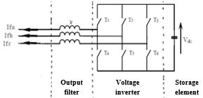
The Figure 1 shows the power circuit of the parallel active filter with a voltage structure. This filter is composed with a voltage inverter, an output filter (lf), and a storage element.
Figure 1. Power circuit of a parallel active filter with a voltage structure
4.1 The voltage inverter
The voltage inverter is a controlled IGBT three-phase voltage inverter. The control of two IGBTs of the same arm is done in a complementary way, that is to say, if the first IGBT is open the other is closed and vice versa. With this principle, the opening and closing sequences depend on the state of the control signals (Sa, Sb, Sc) given by the Eqns. (8), (9) and (10).
$S_{a}=\left\{\begin{array}{l}1 \text { If : } T_{1} \text { is close and } T_{4} \text { is open } \\ 0 \text { If }: T_{4} \text { is close and } T_{1} \text { is open }\end{array}\right\}$ (8)
$\mathrm{S}_{\mathrm{b}}=\left\{\begin{array}{l}1 \text { If }: \mathrm{T}_{2} \text { is close and } \mathrm{T}_{5} \text { is open } \\ 0 \text { If : } \mathrm{T}_{5} \text { is close and } \mathrm{T}_{2} \text { is open }\end{array}\right\}$ (9)
$\mathrm{S}_{\mathrm{c}}=\left\{\begin{array}{l}1 \text { If : } \mathrm{T}_{3} \text { is close and } \mathrm{T}_{6} \text { is open } \\ 0 \text { If : } \mathrm{T}_{6} \text { is close and } \mathrm{T}_{3} \text { is open }\end{array}\right\}$ (10)
The voltages between each two phases are then defined by the Eq. (11).
$\left[\begin{array}{c}V_{\mathrm{fa}}-V_{\mathrm{fb}} \\ V_{\mathrm{fb}}-V_{\mathrm{fc}} \\ \mathrm{V}_{\mathrm{fc}}-V_{\mathrm{fa}}\end{array}\right]=\left[\begin{array}{l}\mathrm{S}_{\mathrm{a}}-\mathrm{S}_{\mathrm{b}} \\ \mathrm{S}_{\mathrm{b}}-\mathrm{S}_{\mathrm{c}} \\ \mathrm{S}_{\mathrm{c}}-\mathrm{S}_{\mathrm{a}}\end{array}\right] V_{\mathrm{dc}}$ (11)
The voltages Vfa, Vfb and Vfc satisfy the Eq. (12).
$\left[\begin{array}{c}\mathrm{V}_{\mathrm{fa}} \\ \mathrm{V}_{\mathrm{fb}} \\ \mathrm{V}_{\mathrm{fc}}\end{array}\right]=\left[\begin{array}{c}\mathrm{V}_{\mathrm{sa}} \\ \mathrm{V}_{\mathrm{sb}} \\ \mathrm{V}_{\mathrm{sc}}\end{array}\right]+\mathrm{L}_{\mathrm{f}} \frac{\mathrm{d}}{\mathrm{dt}}\left[\begin{array}{c}\mathrm{I}_{\mathrm{fa}} \\ \mathrm{I}_{\mathrm{fb}} \\ \mathrm{I}_{\mathrm{fc}}\end{array}\right]$ (12)
Assuming that the network voltages being to be balanced, and knowing that the sum of the currents injected by the inverter is equal to zero, the Eq. (13) can be written.
$\left\{\begin{array}{c}\mathrm{V}_{\mathrm{sa}}+\mathrm{V}_{\mathrm{sb}}+\mathrm{V}_{\mathrm{sc}}=0 \\ \mathrm{I}_{\mathrm{fa}}+\mathrm{I}_{\mathrm{fb}}+\mathrm{I}_{\mathrm{fc}}=0\end{array}\right.$ (13)
From Eqns. (12) and (13), we can deduce the Eq. (14).
$V_{\mathrm{fa}}+\mathrm{V}_{\mathrm{fb}}+\mathrm{V}_{\mathrm{fc}}=0$ (14)
Substituting Eq. (14) into Eq. (11), the Eq. (15) is got.
$\left[\begin{array}{c}\mathrm{V}_{\mathrm{fa}} \\ \mathrm{V}_{\mathrm{fb}} \\ \mathrm{V}_{\mathrm{fc}}\end{array}\right]=\left[\begin{array}{c}2 \mathrm{~S}_{\mathrm{a}}-\mathrm{S}_{\mathrm{b}}-\mathrm{S}_{\mathrm{c}} \\ -\mathrm{S}_{\mathrm{a}} 2 \mathrm{~S}_{\mathrm{b}}-\mathrm{S}_{\mathrm{c}} \\ -\mathrm{S}_{\mathrm{a}}-\mathrm{S}_{\mathrm{b}} 2 \mathrm{~S}_{\mathrm{c}}\end{array}\right] \frac{\mathrm{V}_{\mathrm{dc}}}{3}$ (15)
Thus, we can express eight output voltages cases. All possibilities are summarized in Table 1.
Table 1. Output voltages
|
Case number |
$\mathbf{S}_{\mathrm{a}}$ |
$\mathbf{S}_{\mathrm{b}}$ |
$\mathbf{S}_{\mathrm{c}}$ |
$\mathbf{V}_{\mathrm{fa}}$ |
$\mathbf{V}_{\mathrm{fb}}$ |
$\mathbf{V}_{\mathrm{fc}}$ |
|
0 |
0 |
0 |
0 |
0 |
0 |
0 |
|
1 |
1 |
0 |
0 |
$\frac{2 \mathrm{~V}_{\mathrm{dc}}}{3}$ |
$\frac{-V_{\mathrm{dc}}}{3}$ |
$\frac{-V_{\mathrm{dc}}}{3}$ |
|
2 |
0 |
1 |
0 |
$\frac{-V_{\mathrm{dc}}}{3}$ |
$\frac{2 V_{\mathrm{dc}}}{3}$ |
$\frac{-V_{\mathrm{dc}}}{3}$ |
|
3 |
1 |
1 |
0 |
$\frac{V_{\mathrm{dc}}}{3}$ |
$\frac{V_{\mathrm{dc}}}{3}$ |
$\frac{-2 \mathrm{~V}_{\mathrm{dc}}}{3}$ |
|
4 |
0 |
0 |
1 |
$\frac{-V_{\mathrm{dc}}}{3}$ |
$\frac{-V_{\mathrm{dc}}}{3}$ |
$\frac{2 V_{\mathrm{dc}}}{3}$ |
|
5 |
1 |
0 |
1 |
$\frac{V_{\mathrm{dc}}}{3}$ |
$\frac{-2 \mathrm{~V}_{\mathrm{dc}}}{3}$ |
$\frac{V_{\mathrm{dc}}}{3}$ |
|
6 |
0 |
1 |
1 |
$\frac{-2 \mathrm{~V}_{\mathrm{dc}}}{3}$ |
$\frac{V_{\mathrm{dc}}}{3}$ |
$\frac{V_{\mathrm{dc}}}{3}$ |
|
7 |
1 |
1 |
1 |
0 |
0 |
0 |
4.2 The output filter
The role of the output (decoupling) filter is to connect the voltage inverter to the electrical network [18]. Although it limits the dynamics of the current, this filter reduces, in the electrical network, the propagation of components due to switching.
4.3 The storage element
The energy storage in the direct current side is often done by a capacitive storage system represented by a capacitor which plays the role of a DC voltage source [19]. The storage system parameters choice affects dynamics and quality of the parallel active filter compensation. Indeed, a high DC voltage source improves the dynamics of the active filter. In addition, the DC voltage ripples caused by the currents generated by the active filter and limited by the capacitor choice, can degrade the compensation quality of the parallel active filter. These fluctuations are more and more important as the filter current amplitude is large and its frequency is low [20].
In this part, we used the hysteresis control because it offers better static and dynamic compensation performance [21]. The principle of the hysteresis control is shown in Figure 2.
The purpose of hysteresis control, still known under the name of the on/off control, is to control the compensation currents by forcing them to follow those of reference.
Figure 2. Principle of the hysteresis control [22]
Figure 3. Simplified model of the hysteresis band controller [20]
The signals in the output of a hysteresis comparator are used to control the switching order of the switches of each arm composing the inverter.
The control by hysteresis permit to control a converter by indirectly controlling its average switching frequency. This command is based on knowledge of the converter state and establishment of an easy-to-implement switching choice rules [23]. The Figure 3 illustrates the simplified model of the hysteresis band controller.
The hysteresis technique is part of non-linear controls because it works in the principle of all or nothing. This technique has great advantages in terms of robustness and simplicity of implementation. It has a fast response time in dynamic mode, satisfactory stability and precision and moreover automatically limits the current.
The only regulation parameter in the hysteresis command is the band width which determines the error in the currents and the switching frequency.
The hysteresis band regulation technique is one of the most appropriate methods for various applications of current-controlled inverters such as electric drives and active filters [24].
6.1 Impact of a non-linear load
The presence of non-linear loads causes injection of a huge quantity of harmonics in the electrical distribution networks. These harmonics cause high disturbances [25, 26] and distort the shape of the source current witch is not sinusoidal [27, 28].
The simulation parameters of the electrical network and the non-linear load are gathered in Tables 2 and 3.
Table 2. Parameters of the electrical network
|
Parameter |
$V_{s}(V)$ |
f(Hz) |
$\mathrm{R}_{\mathrm{s}}$(Ω) |
$\mathrm{L}_{\mathrm{s}}$(H) |
|
Value |
220 |
50 |
0.001 |
0.006 |
Table 3. Parameters of the non-linear load
|
Parameter |
$\mathrm{R}_{\mathrm{d}}$(Ω) |
$\mathrm{L}_{\mathrm{d}}$(H) |
|
Value |
20 |
0.007 |
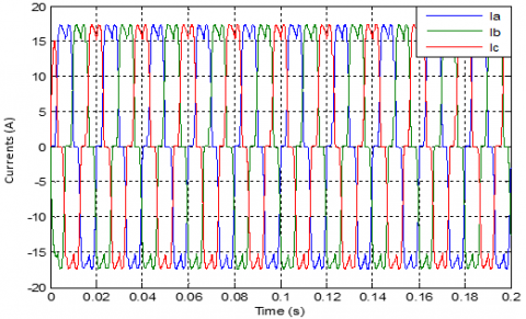
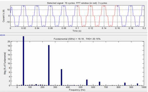
The Figure 4 illustrates the currents shapes for each phase in the presence of a polluting load (rectifier) that generates a large amount of harmonic currents [29, 30].
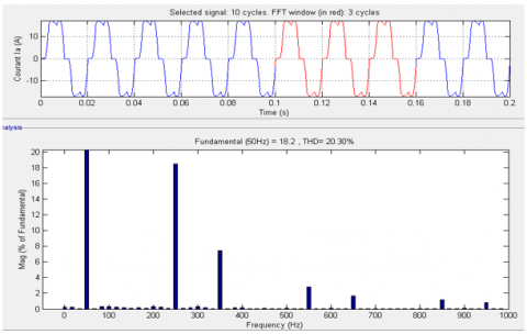
Figure 5. THD of the current Ia
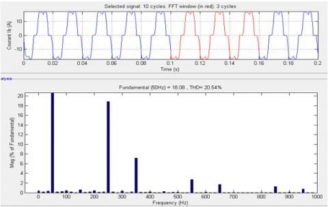
Figure 6. THD of the current Ib
Figure 7. THD of the current Ic
The obtained results show that the currents and voltages for each phase are alternating but polluted with an increase in the maximum value of the current compared to that obtained before addition of the three-phase rectifier.
The Figures 5, 6 and 7 show the spectral analysis of the current absorbed by the load carried out in the three phases after the rectifier addition. The total harmonic distortion (THD) calculation makes possible to discover the harmonics presence in an electrical network. When the THD is equal to zero, it can be said that there are no harmonics in the network.
The Figures 5, 6 and 7 show appearance of harmonic currents since the rectifier is considered as a non-linear load. Indeed, the spectral analysis of the currents absorbed by the load proves presence, in addition to the fundamental (first order), of multiple harmonics. For the THDs, they are equal to: 20.30%, 20.54% and 20.15% for each phase.
6.2 Harmonics filtering
In this part, we present the simulation results of the harmonic pollution decontamination of an electrical network by using a parallel active filter, based on a voltage inverter controlled by the instantaneous powers method The filter parameters are shown in Table 4.
Table 4. Parameters of the parallel active filter
|
Parameter |
$V_{\mathrm{dc}}$(V) |
$\mathrm{R}_{\mathrm{f}}$(Ω) |
$L_{f}$(H) |
$C_{d c}$(F) |
|
Value |
500 |
5 |
0.002 |
0.3 |
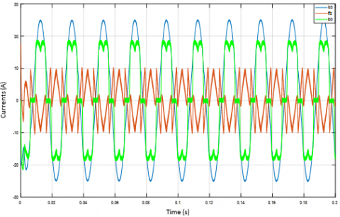
Figure 8. Source, load and parallel active filter currents waveforms for the phase «a»
Figure 9. Source, load and parallel active filter currents waveforms for the phase «b»
Figure 10. Source, load and parallel active filter currents waveforms for the phase «c»
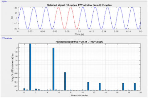
Figure 11.THD of the current Ia after filtering
Figure 12. THD of the current Ib after filtering
The Figures 8, 9 and 10 present the waveforms of the source, load and parallel active filter currents for different phases.
After injection of the reference current (obtained by the real and imaginary instantaneous power method [31, 32]) produced by the active filter, we can see that the source current is now sinusoidal and free of all harmonic disturbances. Therefore, a sinusoidal three-phase source current is obtained.
Figure 13. THD of the current Ic after filtering
Table 5. THDs values before and after harmonics filtering
|
|
THD (%) |
|
|
Before filtering |
After filtering |
|
|
Phase «a» |
20.30 |
2.52 |
|
Phase «b» |
20.54 |
2.51 |
|
Phase «c» |
20.15 |
2.51 |
The Figures 11, 12 and 13 present a spectral analysis of the source current carried out in the three phases after filtering.
The spectral representations shown in Figures 11, 12 and 13 confirm reduction of harmonics in the source currents. In fact, the THDs values goes from 20.30%, 20.54% and 20.15% before filtering, to 2.52%, 2.51% and 2.51% after filtering. These results confirm the strategy followed for reducing harmonics. The Table 5 summarizes the THDs comparison before and after harmonics filtering.
The work presented in this paper is one of the modern solutions based on power electronics to remedy problem of harmonic pollution. To improve energy quality of an electrical network, a parallel active filter (current filtering) based on a two-level voltage inverter controlled by the hysteresis technique was selected.
In order to assess ability of the chosen parallel active filter, two main steps were followed: the first step is the harmonic currents detection using the instantaneous real and imaginary powers which directly gives the shape of harmonic wave to be compensated, and has an adequate response for tracing varying harmonics over time [20]. The second step is the THDs values calculation for each phase.
The different obtained results confirm effectiveness of the introduced active filter by reducing the THDs before filtering compared to those after filtering.
As perspectives, we propose:
- The use of the FACT systems to filter, in the same time, the voltage and current harmonics.
- The application of intelligent techniques such as neural networks and fuzzy logic to filter harmonics.
|
AC |
Alternative Current |
|
DC |
Direct Current |
|
Vs |
Voltage of the AC source |
|
Vdc |
Voltage of the DC bus |
|
Rs |
Resistance of the AC source |
|
Ls |
Inductance of the AC source |
|
Rd |
Resistance of the non-linear load |
|
Ld |
Inductance of the non-linear load |
|
Rf |
Resistance of the parallel active filter |
|
Lf |
Inductance of the parallel active filter |
|
Cdc |
Capacitor of the DC bus |
[1] Dzonde Naoussi, S.R. (2011). Implantation of neuromimetic networks on FPGA target application to the integration of an active filtering system. Ph.D. dissertation. University of Strasbourg, France.
[2] Chaoui, A. (2010). Three-phase active filtering for non-linear loads. Ph.D. dissertation. University of Setif, Algeria.
[3] Bermeo, A.L.D. (2006). Advanced system controls dedicated to improving power quality: from low voltage to voltage rise. Ph.D. dissertation. National Polytechnic Institute of Grenoble, France.
[4] Akagi, H. (1997). Control strategy and site selection of a shunt active filter for damping of harmonic propagation in power distribution systems. IEEE Transactions on Power Delivery, 12(1): 354-363. https://doi.org/10.1109/61.568259
[5] Al-Zamil, A.M., Torrey, D.A. (2000). Harmonic compensation for three-phase adjustable speed drives using active power line conditioner. In 2000 Power Engineering Society Summer Meeting (Cat. No. 00CH37134, Seattle, WA, USA, pp. 867-872. https://doi.org/10.1109/PESS.2000.867471
[6] Nava-Segura, A., Mino-Aguilar, G. (2000). Four-branches-inverter-based-active-filter for unbalanced 3-phase 4-wires electrical distribution systems. In Conference Record of the 2000 IEEE Industry Applications Conference. Thirty-Fifth IAS Annual Meeting and World Conference on Industrial Applications of Electrical Energy (Cat. No. 00CH37129), Rome, Italy, pp. 2503-2508. https://doi.org/10.1109/IAS.2000.883174
[7] Saitou, M., Matsui, N., Shimizu, T. (2003). A control strategy of single-phase active filter using a novel DQ transformation. In 38th IAS Annual Meeting on Conference Record of the Industry Applications Conference, Salt Lake City, UT, USA, pp. 1222-1227. https://doi.org/10.1109/IAS.2003.1257706
[8] Kumar, S., Umamaheswari, B. (2008). Real time implementation of active power filters for harmonic suppression and reactive power compensation using dSPACE DS1104. Journal of Electrical Engineering and Technology, 3(3): 373-378. https://doi.org/10.5370/JEET.2008.3.3.373
[9] Hooshmand, R.A., Esfahani, M.T. (2011). A new combined method in active filter design for power quality improvement in power systems. ISA Transactions, 50(2): 150-158. https://doi.org/10.1016/j.isatra.2010.12.001
[10] Ketabi, A., Farshadnia, M., Malekpour, M., Feuillet, R. (2013). A new control strategy for active power line conditioner (APLC) using adaptive notch filter. Electrical Power and Energy Systems, 47: 31-40. https://doi.org/10.1016/j.ijepes.2012.10.063
[11] Sharmeela, C., Mohan, M.R., Uma, G., Baskaran, J. (2007). Fuzzy logic controller based three phase shunt active filter for line harmonics reduction. Journal of Computer Science, 3(2): 76-80.
[12] Akagi, H., Kanazawa, Y., Nabae, A. (1984). Instantaneous reactive power compensator comprising switching devices without energy storage components. IEEE Transactions on Industry Applications, IA-20(3): 625-630. https://doi.org/10.1109/TIA.1984.4504460
[13] Ignatova, V. (2006). Methods for analyzing quality of the electrical energy, application to voltage dips and harmonic pollution. Ph.D. dissertation. University of Grenoble, France.
[14] Hamidi, A., Rahmani, S., AI-Haddad, K. (2007). A Novel Hybrid Series Active Filter for Power Quality Compensation. IEEE Power Electronics Specialists Conference, Orlando, USA, pp. 1009-1104. https://doi.org/10.1109/PESC.2007.4342146
[15] Bergeras, F. (2010). Study of new active filter structures integrated in microwaves. Ph.D. dissertation. University of Limoges, France.
[16] Boukadoum, A., Bahi, T. (2014). Harmonic current suppression by shunt active power filter using fuzzy logic controller. Journal of Theoretical and Applied Information Technology, 68(3): 651-656. https://doi.org/10.1109/ISIE.2011.5984186
[17] Akagi, H., Kanazawa, Y., Nabae, A. (1983). Generalized theory of the instantaneous reactive power in three-phase circuits. International Power Electronics Conference, Tokyo, Japan, pp. 1375-1386.
[18] Join, C. (2002). Diagnosis of non-linear systems, contribution to decoupling methods. Ph.D. dissertation. University of Nancy 1, France.
[19] Ould Abdeslam, D., Wira, P., Merckle, J., Chapuis, Y.A., Flieller, D. (2006). Neuromimetic strategy for identifying and controlling a parallel active filter. International Journal of Electrical Engineering, 9(1): 35-64.
[20] Chelli, Z., Toufouti, R., Omeiri, A., Saad, S. (2015). Hysteresis control for shunt active power filter under unbalanced three-phase load conditions. Journal of Electrical and Computer Engineering, 2015: 15. https://doi.org/10.1155/2015/391040
[21] Joseph, D., Kalaiarasi, N., Rajan, K. (2015). A novel reference current generation algorithm for three phase shunt active power filter. Journal of Power Electronics and Renewable Energy Systems, pp. 1467-1475. https://doi.org/10.1007/978-81-322-2119-7_143
[22] Hendawi, E., Khater, F., Shaltout, A. (2010). Analysis, simulation and implementation of space vector pulse width modulation inverter. Proceedings of the 9th WSEAS International Conference on Applications of Electrical Engineering, Malaysia, pp. 124-131.
[23] Moigne, P.L., Delarue, P., Fernandez, S. (2014). Modulation by current hysteresis with state memory of a two-level three-phase inverter. Electrical Engineering Symposium, Cachan, France.
[24] Beaulieu, S. (2007). Study and development of an active harmonic filter in order to improve the quality of the electrical power supply. Master's dissertation. University of Quebec, Canada.
[25] Ghorbani, M.J., Mokhtari, H. (2015). Impact of harmonics on power quality and losses in power distribution systems. International Journal of Electrical & Computer Engineering, 5(1): 166-174. https://doi.org/10.11591/ijece.v5i1.7165
[26] Collocott, C.L., Awodele, K.O., Adebayo, A.V. (2020). Harmonic emission of non-linear loads in distribution systems computer. In Proceedings of the 2020 International SAUPEC/RobMech/PRASA Conference, Cape Town, South Africa, pp. 1-6. https://doi.org/10.1109/SAUPEC/RobMech/PRASA48453.2020.9041104
[27] Francisco, C. (2017). Harmonics, Power Systems, and Smart Grids. CRC Press.
[28] Sivaraman, P., Sharmeela, C. (2021). Power system harmonics. Power Quality in Modern Power Systems, Academic Press.
[29] Hsu, C.Y., Wu, H.Y. (1996). New single-phase active power filter with reduced energy-storage capacity. IEEE Proceedings-Electric Power Applications, 143: 25-30.
[30] You, X.J., Li, Y.D. (2002). A shunt active power filter using dead-beat current control. In IEEE 2002 28th Annual Conference of the Industrial Electronics Society. IECON 02, Seville, Spain, pp. 633-637. https://doi.org/10.1109/IECON.2002.1187581.
[31] Benyettou, L., Tebbakh, M. (2018). Comparison performance five level and seven-level cascaded H-bridge multilevel inverter of total harmonic distortion (THD). Modelling, Measurement and Control A, 91(4): 157-167. https://doi.org/10.18280/mmc_a.910401
[32] Noureddine, S., Morsli, S., Tayeb, A., Mouloud, D. (2021). Optimal fractional-order pi control design for a variable speed PMSG-based wind turbine. Journal Européen des Systèmes Automatisés, 54(6): 915-922. https://doi.org/10.18280/jesa.540615