Achouri Mourad* | Youce Zennir | Cherif Tolba
© 2022 IIETA. This article is published by IIETA and is licensed under the CC BY 4.0 license (http://creativecommons.org/licenses/by/4.0/).
OPEN ACCESS
Inverted pendulum is a well-known problem in the control theory because several systems such as robot balancing, Segway, hover board riding and operation of a rocket propeller are inherently based on Inverted Pendulum, furthermore it possesses a height non-linear and unstable dynamics. The main objective of our study is to introduce a comparative analysis of fuzzy logic (FLC), radial basis function neural network (RBF) and integral sliding mode control (ISMC) tuned with whale optimizer algorithm (WOA) for the control of the angle position and velocity of the inverted pendulum system. The implemented controller schemas can adequately reflect and approximate a certain type of uncertainties, nevertheless their parameters should be fine-tuned in order to get height and efficient performance, therefore all the antecedents and consequences of those controllers were tuned with WOA. This later provide height accuracy and fast convergence with height dimensional cost function. Comparative results shows that ISMC-WOA outperforms other techniques in term of settling time and overshoot.
fuzzy logic, radial basis function neural network, integral sliding mode, whale optimizer algorithm, inverted pendulum, control trajectory
The inverted pendulum system is a famous benchmark model in the control theory because it is unstable, coupled and complex non-linearity model, furthermore several systems such as robots are based on inverted pendulum, and therefore it attracts the attention of automation engineers to test the efficiency and robustness of the controller.
In the contrast of linear control theory, nonlinear control does not possess the universal solutions neither for systems analysis nor for the construction of their controllers. Most nonlinear control theory often needs precise and relevant model of the system therefore the performance of the deterministic approaches will be directly affected by the accuracy of the modeled system. In fact, the obtaining of mathematical model with those requirements is really difficult and complex in most of times [1].
Indeed several studies have been introduced to deal with non-linearity situation [2, 3] such as adaptive and sliding mode control (Isidori [4], Slotine and Li [5], Utkin [6], Drakunov and Utkin [7], Slotine [8, 9] …etc.). However, despite of their robustness and efficiency they still require height knowledge of the derivative and accurate complex dynamics of the system, moreover the model is just an approximation of real world.
Other effective method is fuzzy logic controller (FLC). FLC was firstly developed by lotfizeddah in 1965 it is based on human expertise. It describes a real world with a simple set of linguistic variables (spoken or non-numeric) rather than crisp logic (0-1) just like humans thinking [10], hence it can approximate systems with a set of linguistic variables without knowing the mathematical model of the system concerned. Since the first application of mamdani [11] on steam engines, FLC have gained a proliferating interest in several industrial fields. This is due to its simplicity and its performance to reflect uncertainties [1, 11]. Nevertheless, the application of FLC in some pertinent areas have been limited by its lack of systematic design and soliciting knowledge of experts [12, 13].
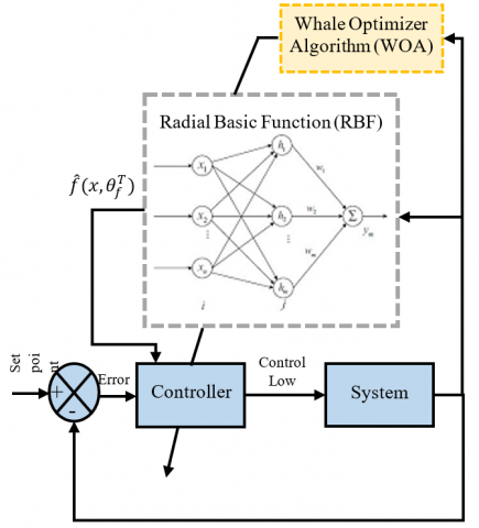
The RBF neural network control algorithm has gathered a lot of concern regarding its ability to be adopted in many control strategies. It can be employed in the tuning process via the back-propagation algorithm (determining the parameters of PID or any given controller), furthermore it can successfully approximate any nonlinear function or parameter and it can also apply as a filter or address uncertainties.
Other proliferating areas that can alleviate the main drawbacks of FLC is meta-heuristic schema. Meta-heuristic is an optimization technique, which seeks for a best or near optimal variable (minimum for minimization problem or maximum for maximization problem) within, given search space and many approaches have been proposed. Whale optimizer algorithm (WOA) is a recent met-heuristic method inspired from a social behavior of humpback whale, which mimics their hunting mechanism (bubble-net). This algorithm is able to handle functions with several local minima in height dimensional space, moreover it provides height accuracy and fast convergence.
The rest of the paper is organized as follows. Section 2 provide the related work. In Section 3 gives main model of the inverted pendulum. The proposed meta-heuristic algorithm is explained in Section 4 and its subsections. The RBF based neural network and ISMC controller are both explained in Section 5 and 6. Section 7 presents the main parameters of the WOA used to find the near optimal parameters of the applied control strategies. Finally, in Sections 8 and 9 results and conclusions are explained respectively.
Meta-heuristic schema based fuzzy logic tuning process and the control of inverted pendulum have been studied extensively in the literature. Amador et al. [14]. They introduced Chicken Search Optimization (CSO) to design the optimal parameter of fuzzy logic controller and this later was applied to two benchmark model (inverted pendulum and Water Tank Controller). Bejarbaneh et al. [15] introduced a hybrid PSO search technique called PSOSCALF to determine the best parameters of PID type fuzzy logic. This proposed schema is applied to the control of nonlinear Inverted Pendulum (IP) system. Rabah et al. [16] investigate the performance of PID, fuzzy logic and fuzzy PID controller to stabilize the gyroscopic inverted pendulum. PID controller, fuzzy logic controller and PID-type Fuzzy adaptive controller approaches are applied to retain the pendulum on the linear moving car vertically and to stabilize the car on the equilibrium position for real-time control [17]. In their study Lakmesari et al. [18] combined feedback linearization (FL) and sliding mode controller (SMC) this proposed schema is improved by fuzzy rules and gradient descent laws then the coefficients are determined by termed multi-objective ant lion optimizer (MOALO) and finally this technique is implemented to control a fourth-order under-actuated nonlinear inverted pendulum system. Ghaliba and Oglah [19] designed the parameters of fuzzy-like PID (FPID) controller with genetic algorithm (GA), ant colony optimization (ACO), and social spider optimization (SSO) for the control trajectory of inverted pendulum. Alimoradpour et al. [20] attempt to set fuzzy rules and their membership function and the length of the learning process with genetic algorithm and the results of the proposed method on inverse pendulum was promising. In the first phase of their studies Magdy et al. [21] presented a model of inverted pendulum regarding to Alembert’s principle then they verified this model with other after that they compared the results of PID-GSA and PID-GA controller on this model. Erkol [22] presented a fractional order PID controller for the position control of a two wheeled inverted pendulum and compared the performance of artificial bee colony, particle swarm optimization, grey wolf optimizer, and cuckoo search algorithm in finding the best parameter of this controller. Abdullah et al. [23] employed Linear Quadratic Regulator (LQR) to stabilize a Three Links Inverted Pendulum with Cart and parameters was determined with the help of Genetic Algorithm (GA).
Motivated by above-mentioned discussion our study aims to present a comparative study of FLC, RBF and ISMC and determine their parameters with the help of WOA. All the proposed schemas have been implemented on the control trajectories of the inverted pendulum. The comparison is carried out based on various parameters like time and steady error. The results prove the efficiency of the different proposed methodologies, however the ISMC was the outstanding one in term of settling time and steady error.
The inverted pendulum is governed by the following differential equations [5]:
$\left\{\begin{array}{c}\dot{x}_{1}=x_{2} \\ \dot{x}_{2}=\frac{g \cdot \sin x_{1}-\frac{m \cdot l \cdot x_{2}^{2} \cdot \cos x_{1} \cdot \sin x_{1}}{m_{c}+m}}{l\left(\frac{4}{3}-\frac{m \cdot \cos x_{1}^{2}}{m_{c}+m}\right)}+\frac{\frac{\cos x_{1}}{m_{c}+m}}{l\left(\frac{4}{3}-\frac{m \cdot \cos x_{1}^{2}}{m_{c}+m}\right)} u\end{array}\right.$ (1)
where, x1=θ is the angle of rotation, $x_{2}=\dot{\theta}$ the angular velocity, g=9.81m/s2 the acceleration due to gravity, $m_{c}$ the mass of the trolley, m the mass of the beam, 2.l the length of the beam, u the force (command) applied to the system.
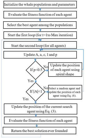
WOA is relatively new meta-heuristic schema firstly proposed by Seyed Ali Mirjalili in 2016. This algorithm imitates the hunting mechanism of humpback whales, which describe the bubble-net technique with simple mathematical model. The essential of the proposed algorithm can be performed in 3 main phases, which are encircling prey, attacking prey (exploitation phase) and searching prey (exploration phase). In the encircling and search phase the humpback whales consider the agent with best score or random agent (to skip from local minima) as a target point thus it update their position within the neighborhood of this position. After defining the best candidate the humpbacks moves either with circular or spiral (see section 4.2) shape toward the target point (see Figure 1).
Figure 1. Flowchart of WOA
4.1 Encircling
Initially after finding the prey the humpback whales start the encircling process, however the optimal position within a given search space is not known hence this algorithm consider the current best agent as the prey position (optimal solution), then the remain candidate will update their position according to the best solution (best candidate). The main mathematical model of the encircling phase is given by Eq. (2), (3):
$\vec{D}=\left|\vec{C} \cdot \overrightarrow{X^{*}}(t)-\vec{X}(t)\right|$ (2)
$\vec{X}(t+1)=\overrightarrow{X^{*}}(t)-\vec{A} \cdot \vec{D}$ (3)
where, t is the current iteration, $\vec{A}$ and $\vec{C}$ are coefficient vectors, $\overrightarrow{X^{*}}$ represent the position vector of the best candidate, $\vec{X}$ indicate the position vector. It is important to notice that $\overrightarrow{X^{*}}$ must be updated in each iteration if better solution exist.
The coefficient vectors $\vec{A}$ and $\vec{C}$ are provided in Eq. (4), (5):
$\vec{X}(t+1)=\overrightarrow{X^{*}}(t)-\vec{A} \cdot \vec{D}$ (4)
$\vec{X}(t+1)=\overrightarrow{X^{*}}(t)-\vec{A} \cdot \vec{D}$ (5)
where, $\vec{A}$ decrease linearly from 2 to 0 over the course of iterations (in both exploration and exploitation phases) and $\vec{r}$ is a random vector in [0,1]. It is worthy to notice that A defines whether the candidate move toward best agent (when $|\vec{A}|$ >1) or moves far from it when $|\vec{A}|$ <1.
4.2 Attacking prey (bubble-net)
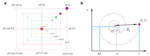
This step is devoted to describe bubble-net strategy. It should be kept in mind that humpback whales attack and encircle their prey simultaneously with shrinking circle and spiral shaped movement toward the prey (target point) when $|\overrightarrow{\mathrm{A}}|<1$ (see Figure 2). In order to simulate this kind of behavior this algorithm proposes 50% probability to choose between this kind of movement. The bubble-net mechanism is given in Eq. (6):
$\left\{\begin{array}{c}\overrightarrow{X^{*}}(t)-\vec{A} \cdot \vec{D} i f p<0.5 \\ \overrightarrow{D^{\prime}} \cdot e^{b l} \cdot \cos (2 \pi l)+\overrightarrow{X^{*}}(t) i f p \geq 0.5\end{array}\right.$ (6)
where, $\overrightarrow{D^{\prime}}=\left|\overrightarrow{X^{*}}(t)-\vec{X}(t)\right|$ represent the distance of the i-th whale to the prey (best solution obtained so far), b is a constant for defining the shape of the logarithmic spiral, l is a random number in [-1,1], and p is a random number in [0,1].
(a) shrinking circle movement (b) spiral shaped movement [24]
Figure 2. Attacking prey mechanism
4.3 Searching prey (exploration)
Regarding to the variation of the vector $\overrightarrow{\mathrm{A}}$ this step investigates the exploration ability of this algorithm. In reality, the humpback whale randomly moves to the target based on the position of each other. For the sake of describing the exploration, process the search agent moves far away the target (reference whale) when the value of $\overrightarrow{\mathrm{A}}$ is less than -1 or greater than 1. In the contrary of exploitation, phase each candidate update their position with respect to a randomly chosen agent (when $|\vec{A}|$ >1) in exploration mechanism. This phase is expressed in Eq. (7), (8).
$\vec{D}=\mid \vec{C}$.$\overrightarrow{X_{\text {rand }}}-\vec{X}$ (7)
$\vec{X}(t+1)=\overrightarrow{X_{\text {rand }}}-\vec{A} \cdot \vec{D}$ (8)
where, $\overrightarrow{X_{\text {rand }}}$ indicates a random position vector (a random whale) chosen from the current population [24].
The radial basis function (RBF) neural network is a multilayer neural network, which usually adopts three-layer feed-forward to map rapidly the inputs to output by adjusting its weights (online adjustment) and making the feedback control tend to zero [25].
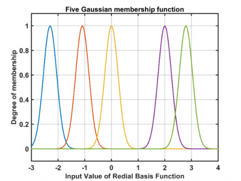
RBF neural network takes input r(k), radial basis function vector in hidden layer H=[h1, ….., hm]Tand adopt a Gaussian membership as an activation function, which is given in Eq. (9):
$h_{j}=\exp\left(\frac{\left\|r(k)-C_{j}\right\|}{2 b_{j}^{2}}\right)$ (9)
where, j=1, .., m, Cj, bj denotes respectively the center and the width vector of the Gaussian membership function of the nod j.
The weight of RBF are written in Eq. (10):
$W=\left[w_{1}, \ldots, w_{2}\right]^{T}$ (10)
Then its output is expressed in Eq. (11):
$y(t)=h_{1} w_{1} \ldots+h_{j} w_{j}+\ldots+h_{m} w_{m}$ (11)
5.1 Controller design
The Eq. (1). can be represented by the following double integrator system:
$\ddot{x}=f(x, \dot{x})+g(x, \dot{x}) u$ (12)
Considering that, the errors of system expressed in Eq. (13):
$e=y_{d}-y, S=\left[\begin{array}{ll}e & \dot{e}\end{array}\right]^{T}$ (13)
where, yd is the desired input, e and è are the error and the derivative of error.
Consequently, the control objective is now modified to design the control input u, so that the closed loop system written in Eq. (12). errors S converge to zero in finite time.
The control law can be formulated as given in Eq. (14):
$u=\frac{1}{g(x)}\left(-f(x)+\ddot{y}_{d}+K^{T} S\right)$ (14)
where, $K=\left[\begin{array}{ll}k_{p} & k_{d}\end{array}\right]^{T}$ is designed such that the polynomial $s^{2}+k_{d} s+k_{p}=0$ is in the left side of the complex plane, which ensure the convergence of e and $\dot{e}$ to zero in finite time.
Now after using the RBF to approximate the unknown function f(x) the control law can be rewritten as given in Eq. (15) and the unknown function is provided in Eq. (16):
$u=\frac{1}{g(x)}\left(-\hat{f}\left(x, \theta_{f}\right)+\ddot{y}_{d}+K^{T} S\right)$ (15)
$\hat{f}\left(x, \theta_{f}\right)=\theta_{f}^{T} h(x)$ (16)
where, h(x) is Gaussian function, $\theta_{f}^{T}$ is the vector of the adjustable parameters of the function $\hat{f}$.
5.2 Stability analysis
We define the vector of the optimal parameter $\theta_{f}^{*}$ expressed in Eq. (17) by:
$\theta_{f}^{*}=\operatorname{argmin}_{\theta_{f \in \Omega_{f}}}\left(\sup _{x \in U_{c}}\left|\hat{f}\left(x, \theta_{f}\right)-f(x)\right|\right)$ (17)
where,
$f(x)=\theta_{f}^{* T} h(x)+\varepsilon_{1}$ (18)
where, ε1 is the minimum approximation error for f.
$\hat{f}\left(x, \theta_{f}\right)-f(x)=\theta_{f}^{T} h(x)-\theta_{f}^{* T} h(x)+\varepsilon_{1}=\tilde{\theta}_{f}^{T} h(x)+\varepsilon_{1}$ (19)
where,
$\tilde{\theta}_{f}^{T}=\theta_{f}^{T}-\theta_{f}^{* T}$ (20)
Now, we substitute the control law written in Eq. (15, 12). we get:
$\ddot{e}=-K^{T} S+\left[\hat{f}\left(x, \theta_{f}\right)-f(x)\right]$ (21)
Assuming that:
$A=\left[\begin{array}{cc}0 & 1 \\ -k_{p} & -k_{d}\end{array}\right], B=\left[\begin{array}{l}0 \\ 1\end{array}\right]$ (22)
Now, Eq. (21) Can be rewritten as given in Eq. (23):
$\dot{S}=A S+B\left[\hat{f}\left(x, \theta_{f}\right)-f(x)\right]$ (23)
Submitting the control law given by Eq. (19) into Eq. (23) we find:
$\dot{S}=A S+B\left[\tilde{\theta}_{f}^{T} h(x)+\varepsilon_{l}\right]$ (24)
Now, we define the Lyapunov candidate function in Eq. (25):
$V=\frac{1}{2} S^{T} P S+\frac{1}{2 \gamma_{f}} \tilde{\theta}_{f}^{T} \tilde{\theta}_{f}$ (25)
where, $\gamma_{f}$ is positive constant. P is a positive definite and symmetric matrix, which satisfies the following Lyapunov equation:
$A^{T} P+P A=-Q$ (26)
with, Q≥0 and A is given Eq. (22).
By deriving the Lyapunov function and substituting the Eq. (24) and Eq. (26) we obtain:
$\dot{V}=-\frac{1}{2} S^{T} Q S+S^{T} P B\left[\tilde{\theta}_{f}^{T} h(x)+\varepsilon_{1}\right]+\frac{1}{\gamma_{f}} \tilde{\theta}_{f}^{T} \dot{\tilde{\theta}}_{f}$ (27)
$\dot{V}=-\frac{1}{2} S^{T} Q S+\left(S^{T} P B h(x)+\frac{1}{\gamma_{f}} \dot{\tilde{\theta}}_{f}\right) \tilde{\theta}_{f}^{T}+S^{T} P B \varepsilon_{l}$ (28)
We choose $\dot{\tilde{\theta}}_{f}=-\gamma_{f}\left(S^{T} P B h(x)\right)$ and we submit into Eq. (28). we get:
$\dot{V}=-\frac{1}{2} S^{T} Q S+S^{T} P B \varepsilon_{1}$ (29)
Since $-\frac{1}{2} S^{T} Q S<0$, if we design $\varepsilon_{1}$ very small by using RBF, we will get $\dot{V}<0$. Then we can get that S and $\tilde{\theta}_{f}$ are bounded. And by invoking the barbarat’s lemma we can ensure the convergence.
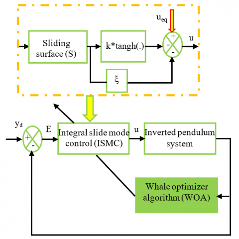
The ISMC adopt the same schema as sliding mode control (SMC), in which its control law is established by two term the first is the equivalent control, which attempt to bring the system dynamics to a given sliding surface while the second term is the switched control, which seeks to retain the dynamics of system along sliding surface. The only difference is that the integral term is added to the sliding surface for the sake of obtaining better performance (fast convergence, reduce the chattering phenomenon, minimize the cost function ...etc.) [2].
6.1 Controller design
In ISMC the sliding surface is represented in Eq. (30). Which is given by:
$S=\left(\frac{d}{d t}+\lambda\right)^{n-1} e+z$ (30)
with, $z=k_{p} e+k_{i} \int e$ is the integral term (kp and ki are respectively the proportional and integral gain), e=yd-y is the error (yd is the desired trajectory and y is the output of the system), n represent the order of the system and λ indicates a positive constant.
Given that n=2 the sliding surface can be rewritten as in Eq. (31):
$S=\dot{e}+\lambda e+z$ (31)
The objective control of ISMC is to design two-control law, which are equivalent control ueq and switched control udis. The first controller seeks to bring the system’s dynamics to the desired sliding surface by making $\dot{S}=0$, while the second attempt to retain this later in a given sliding surface. After deriving the sliding surface and considering the Eq. (12). we obtain the following equation:
$\dot{S}=\ddot{e}+\lambda \dot{e}+\dot{z}=\ddot{y}_{d}-f(x, t)-g(x, t) u+\lambda \dot{e}+\dot{z}$ (32)
Thus, the equivalent and swished term can be designed as written in Eq. (33). And Eq. (34):
$u_{e q}=\frac{-f(x, t)+\ddot{y}_{d}+\lambda \dot{e}+\dot{z}}{g(x, t)}$ (33)
$u_{d i s}=-k \operatorname{sign}(S)-\xi S$ (34)
where, sign(S) represents the sign function, k and ξ are a positive constant.
6.2 Stability analysis
In order, to investigate the stability of the proposed controller we have considered the following Lyapunov function given in Eq. (35):
$V=\frac{1}{2} S^{2}$ (35)
After taking the derivative of Eq. (35). and replacing the equivalent and switched control written in Eq. (33), (34) we find:
$\dot{V}=S \dot{S}$ (36)
$\dot{V}=S\left(\ddot{y}_{d}-f(x, t)-g(x, t) u+\lambda \dot{e}+\dot{z}\right)$ (37)
$\dot{V}=S(-k \operatorname{sig} n(S)-\xi S)$ (38)
$\dot{V} \leq-k|S|-\xi S^{2}$ (39)
Given that $\dot{\mathrm{V}} \leq 0$, thus the system dynamic will converge to the sliding surface in finite time.
The optimizations results involved in the proposed work were carried on MATLAB/Simulink by engaging 25-search agent in 25 iterations for all presented control strategies under the cost function of the mean of root of squared of error (MRSE), which is expressed in Eq. (40):
$M R S E=\sum_{i=1}^{N} e(i)^{2}+\sum_{i=1}^{N}\left(\frac{d e(i)}{d t}\right)^{2}$ (40)
where, e(i) is the error of the trajectory of the i-th sample, $\frac{d e(i)}{d t}$ is derivative of the error for the trajectory of the i-th sample and N is the number of samples.
Figures 3-6 depict the control diagram of the proposed schemas when performing task in order to get the near optimal parameters of those technics.
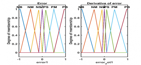
The Takagi Sugono fuzzy logic type have adopted in this work, 14 triangular and trapezoid memberships function was used for the inputs of FLC and the total number of rules is 49 (see Table 1). Since the FLC has 14 memberships function and 49 rules, therefore WOA search for the optimal of the antecedents and consequence parameters of the proposed controller in 12 dimensional space.
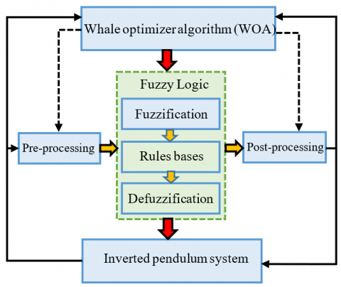
Figure 3. Control strategy of FLC-WOA
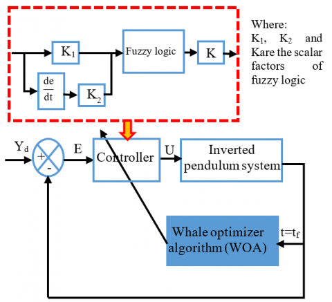
Figure 4. Block diagram of FLC-WOA
Figure 5. Block diagram of RBF-WOA
Figure 6. Block diagram of ISMC-WOA
Table 1. Rule base of FLC
|
e de |
NB |
NM |
NS |
Z |
PS |
PM |
PB |
|
NB |
NB |
NB |
NB |
NB |
NM |
NS |
Z |
|
NM |
NB |
NB |
NB |
NM |
NS |
Z |
PS |
|
NS |
NB |
NB |
NM |
NS |
Z |
PS |
PM |
|
Z |
NB |
NM |
NS |
Z |
PS |
PM |
PB |
|
PS |
NM |
NS |
Z |
PS |
PM |
PB |
PB |
|
PM |
NS |
Z |
PS |
PM |
PB |
PB |
PB |
|
PB |
Z |
PS |
PM |
PB |
PB |
PB |
PB |
The parameters of the applied strategies after performing the optimization are presenter in Figures 7, 8 and Table 2.
Figure 7. Memberships functions of fuzzy logic after optimization by WOA
Figure 8. Memberships functions of RBF after optimization by WOA
Table 2. The parameters of the proposed schema after optimization
|
Parameters |
FLC-WOA |
RBF-WOA |
ISMC-WOA |
|
$k_{p}$ |
10.69 |
40 |
19.48 |
|
$k_{d}$ |
9.53 |
34.99 |
- |
|
$k_{i}$ |
- |
- |
0.69 |
|
$k$ |
13.64 |
- |
0.5 |
|
$\xi$ |
- |
- |
0.5 |
|
$\gamma_{f}$ |
- |
1200 |
- |
|
$\lambda$ |
- |
- |
62.61 |
The objective of the controller is to force the angle of the pendulum θ to follow the desired trajectory defined by: yd=(π/30) sint and the pendulum parameters respectively are: mc=1 kg, m=0.1 kg. The numerical simulation results obtained by the implemented control technics tuned with whale optimizer algorithm for an initial condition of the system x0 = [-0.05, 0] are represented in Figures 9-13.
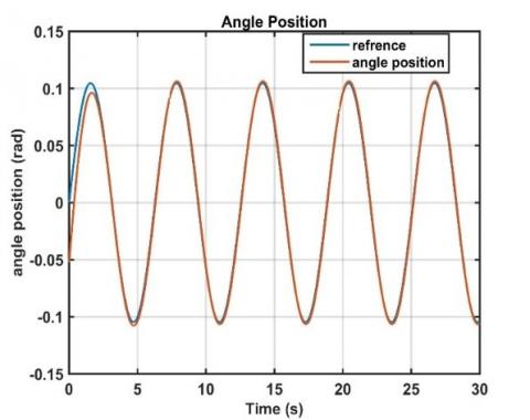
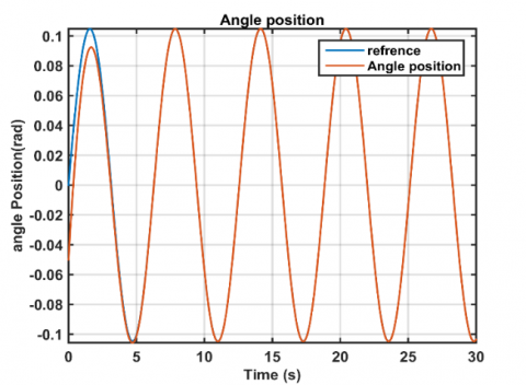
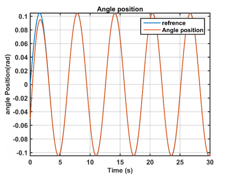
Figure 9-11 highlights the trajectory of angle position obtained by the carried out control strategies, which evidently shows that both trajectory converge rapidly to their respective set point in finite time for both proposed schemas and their performances are summarized in Table 3.
Figure 9. Angle position and the reference trajectory based on FLC-WOA
Figure 10. Angle position and the reference trajectory based on RBF-WOA
Figure 11. Angle position and the reference trajectory based on ISMC-WOA
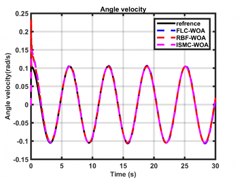
Figure 12. Angle velocity and its reference trajectory based on FLC-WOA, RBF-WOA and ISMC-WOA
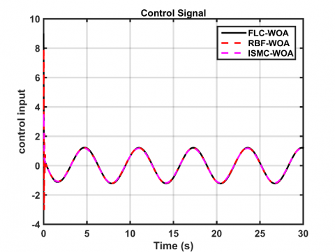
Figure 13. Control input by using FLC-WOA, RBF-WOA and ISMC-WOA laws
Table 3. Performances analysis of control strategies
|
Angle position |
FLC-WOA |
RBF-WOA |
ISMC-WOA |
|
RMSE |
0.0015 |
0.0014 |
0.0014 |
|
Setlling Time (sec) |
3.28 |
2.23 |
2 |
|
Steady Error |
0.003 |
0 |
0 |
|
Overshoot (%) |
0 |
0 |
0 |
Table 3 reports the performances based comparative analysis for the applied control strategy (FLC-WOA, RBF-WOA and ISMC-WOA) on the position of the inverted pendulum. The performance parameters obviously proves that both approaches provide accuracy and shows that the RBF-WOA ISMC-WOA was the outstanding one in term of settling time and steady error.
It is clearer from Figure 12 that the angle velocity rapidly reach its sinusoidal trajectory reference for all control approaches. The FLC-WOA and ISMC-WOA provide height performance with tracking trajectory minimum overshoot as compared to RBF-WOA.
Figure 13 outlines the corresponding simulation results of the control input applied on the inverted pendulum system to achieve a given desired trajectory for the aforementioned schemas and clearly shows that they acquire a sinusoidal, which obviously verifies our claims by obtaining a lesser and continuous signals.
Our study proposed FLC, RBF and ISMC based WOA approach to stabilize the dynamic of inverted pendulum in a given trajectory. The proposed algorithm has the ability to address a non-linear function with height dimensional search space and bypass local minims, furthermore it provides height accuracy and fast convergence. This algorithm is devoted to find near optimal parameters of FLC, RBF and ISMC. The implemented control strategies perfectly reflect the uncertainties and adequately investigate non-linear system. The involved results of the comparative study shows that both strategies provide good performance in the stabilization of the dynamics of inverted pendulum. Overall performance comparison concludes that ISMC over perform other techniques, however the derivatives knowledge and system dynamics should be taken into consideration, and further studies should be move in the direction of adapting the ISMC strategy with FLC and RBF control.
[1] Qiao, F., Zhu, Q., Winfield, A.F., Melhuish, C. (2004). Adaptive sliding mode control for MIMO nonlinear systems based on fuzzy logic scheme. International Journal of Automation and Computing, 1(1): 51-62. https://doi.org/10.1007/s11633-004-0051-4
[2] Irfan, S., Mehmood, A., Razzaq, M.T., Iqbal, J. (2018). Advanced sliding mode control techniques for inverted pendulum: Modelling and simulation. Engineering Science and Technology, An International Journal, 21(4): 753-759. https://doi.org/10.1016/j.jestch.2018.06.010
[3] Khan, S.G., Jalani, J. (2016). Realisation of model reference compliance control of a humanoid robot arm via integral sliding mode control. Mechanical Sciences, 7(1): 1-8. https://doi.org/10.5194/ms-7-1-2016
[4] Isidori, A. (1989). Nonlinear control systems. Springer-Verlag, 105-203.
[5] Slotine, J.J.E., Li, W. (1991). Applied Nonlinear Control. Englewood Cliffs, NJ: Prentice Hall, 199(1).
[6] Utkin, V. (1977). Variable structure systems with sliding modes. IEEE Transactions on Automatic Control, 22(2): 212-222. https://doi.org/10.1109/TAC.1977.1101446
[7] Drakunov, S.V., Utkin, V.I. (1992). Sliding mode control in dynamic systems. International Journal of Control, 55(4): 1029-1037. https://doi.org/10.1080/00207179208934270
[8] Slotine, J.J.E. (1984). Sliding controller design for non-linear systems. International Journal of Control, 40(2): 421-434. https://doi.org/10.1080/00207178408933284
[9] Slotine, J.J. (1987). Applied nonlinear control. Prentice-Hall, Englewood Cliffs, NJ.
[10] Zadeh, L. A. (1965). Information and control. Fuzzy sets. Vol. 8, N°. 3, pp. 338-353.
[11] Mamdani, E.H. (1974). Application of fuzzy algorithms for control of simple dynamic plant. In Proceedings of the Institution of Electrical Engineers, 121(12): 1585-1588. https://doi.org/10.1049/piee.1974.0328
[12] Mourad, A., Zennir, Y. (2022). Fuzzy-PI controller tuned with HBBO for 2 DOF robot trajectory control. Engineering Proceedings, 14(1): 10. https://doi.org/10.3390/engproc2022014010
[13] Achouri, M., Zennir, Y., Tolba, C. (2022). Fuzzy-PI conroller tuned with GWO, WOA and TLBO For 2 DOF robot trajectory control. Algerian Journal of Signals and Systems, 7(1): 1-6. https://doi.org/10.51485/ajss.v7i1.150
[14] Amador-Angulo, L., Castillo, O., Peraza, C., Ochoa, P. (2021). An efficient chicken search optimization algorithm for the optimal design of fuzzy controllers. Axioms, 10(1): 30. https://doi.org/10.3390/axioms10010030
[15] Bejarbaneh, E.Y., Bagheri, A., Bejarbaneh, B.Y., Buyamin, S., Chegini, S.N. (2019). A new adjusting technique for PID type fuzzy logic controller using PSOSCALF optimization algorithm. Applied Soft Computing, 85: 105822. https://doi.org/10.1016/j.asoc.2019.105822
[16] Rabah, M., Rohan, A., Kim, S.H. (2018). Comparison of position control of a gyroscopic inverted pendulum using PID, fuzzy logic and fuzzy PID controllers. International Journal of Fuzzy Logic and Intelligent Systems, 18(2): 103-110. https://doi.org/10.5391/IJFIS.2018.18.2.103
[17] Abut, T., Soyguder, S. (2019). Real-time control and application with self-tuning PID-type fuzzy adaptive controller of an inverted pendulum. Industrial Robot: The International Journal of Robotics Research and Application, 46(1): 159-170. https://doi.org/10.1108/IR-10-2018-0206
[18] Lakmesari, S.H., Mahmoodabadi, M.J., Ibrahim, M.Y. (2021). Fuzzy logic and gradient descent-based optimal adaptive robust controller with inverted pendulum verification. Chaos, Solitons & Fractals, 151: 111257. https://doi.org/10.1016/j.chaos.2021.111257
[19] Ghaliba, A.F., Oglah, A.A. (2020). Design and implementation of a fuzzy logic controller for inverted pendulum system based on evolutionary optimization algorithms. Engineering and Technology Journal, 38(3): 361-374. https://doi.org/10.30684/etj.v38i3A.400
[20] Alimoradpour, S., Rafie, M., Ahmadzadeh, B. (2021). Provide a method based on genetic algorithm to optimize the fuzzy logic controller for the inverted pendulum. https://doi.org/10.21203/rs.3.rs-602450/v1
[21] Magdy, M., El Marhomy, A., Attia, M.A. (2019). Modeling of inverted pendulum system with gravitational search algorithm optimized controller. Ain Shams Engineering Journal, 10(1): 129-149. https://doi.org/10.1016/j.asej.2018.11.001
[22] Erkol, H.O. (2018). Optimal PI Du controller design for two wheeled inverted pendulum. IEEE Access, 6: 75709-75717. https://doi.org/10.1109/ACCESS.2018.2883504
[23] Abdullah, A.I., Alnema, Y.H.S., Thanoon, M.A. (2022). Stabilization of three links inverted pendulum with cart based on genetic LQR approach. Journal Européen des Systèmes Automatisés, 55(1): 125-130. https://doi.org/10.18280/jesa.550113
[24] Mirjalili, S., Lewis, A. (2016). The whale optimization algorithm. Advances in engineering software, 95: 51-67. https://doi.org/10.1016/j.advengsoft.2016.01.008
[25] Gao, H., Li, X., Gao, C., Wu, J. (2021). Neural network supervision control strategy for inverted pendulum tracking control. Discrete Dynamics in Nature and Society, 2021: 5536573. https://doi.org/10.1155/2021/5536573