Mayouf Messaoud
© 2022 IIETA. This article is published by IIETA and is licensed under the CC BY 4.0 license (http://creativecommons.org/licenses/by/4.0/).
OPEN ACCESS
This paper presents a comparative functional analysis of a typical stand-alone photovoltaic system (SPV) with a charging battery. Considering the nonlinear behavior of the PV system, a specific methodology based on Tayler’s expansion series is opted for the modelling, control, and optimization. During the proposed steps, a practical PID controller is designed using a dynamic state space averaging approach. This controller is used to track the maximum power point (MPP) and control the battery charging process. To check the validity of this controller, it is applied with three disparate MPPT algorithms to enhance system performances by preventing drift phenomenon against fast changing in cell temperature and solar irradiance, and control the battery pack to conform with the load rating voltage. A typical 2525 W SPV is simulated in short term to capture fast dynamics transitional details. By comparison with practical manufacturer's specifications of the PV panel, the load, and the battery pack; simulation results show particularly, good performances with fuzzy logic controller in terms of speed tracking, MPPT tracking accuracy, voltage quality, and reducing transient fluctuations. The findings of this research substantiate its efficacy, which may serve as a prototype study for the design and realization of stand-alone photovoltaic systems with energy storage.
drift phenomenon, dynamic state-space averaging model, fuzzy logic, incremental conductance (Inc-Cond), linearization, perturbation and observation (P&O), PID controller, Tayler expansion series
In recent years, electricity production from renewable energy resources has been increasing due to environmental problems and the expected lack of traditional energy sources in the future. In view of the increase in the cost of conventional energy and the limitation of their resources, photovoltaic energy is increasingly becoming a solution among the options promising energy sources with benefits such as: the energy produced is non-polluting, requires little maintenance and inexhaustible [1]. Direct exploitation of PV systems is currently considered cost-effective in a wide range of domestic and technical applications, where they offer irreplaceable service autonomy in remote areas. However, the photovoltaic system still has relatively low conversion efficiency. Indeed, the power delivered by generator depends on the solar irradiance level, the cell temperature, and the load current. Hence, these operating conditions must be assessed in the design of the PV system to perfect the output power either to the standalone electrical-type load or the power company utility grid [2]. At the maximum power point (MPP), the PV generator operates at its highest efficiency. Therefore, to extract the maximum power under varying conditions, various MPPT techniques applied to PV power systems, are reviewed and classified in Precup et al. [2] and Subudhi and Pradhan [3] based on the type of control strategy, circuitry, number of control variables, and cost of applications.
Several contributions are carried out on batteries-free SPV. They are often presented in a comparative study form between conventional and intelligent optimization techniques regarding tracking efficiency, accumulated energy, and tracking drift phenomenon against fast step changes. In the context of comparing the particle swarm optimization algorithm (PSOA) with other techniques, a comparative energy assessment made by Dabra et al. [4] shows that it is more effective than P & O and fuzzy P & O system. However, this technique proved to be less effective compared with cuckoo search algorithm (CSA), in terms of speed tracking, oscillation levels and output power according to Kotla et al. [5]. The studies done in Cheng et al. [6] and Liu et al. [7] reveal that asymmetrical fuzzy logic controller (FLC) based MPPT technique is more significant with good tracking accuracy, comparing with P&O and classical symmetrical FLC-based MPPT techniques. By assessing three typical MPPT algorithms discussed in Li et al. [8], hybrid-step-size Beta method gives the highest tracking efficacy and acquired energy comparing with variable step size incremental conductance (VSS-IncCond) and fixed step size (P&O). Simulation and experimental results referred in Tang et al. [9] show significant enhancement in the tracking accuracy, using fractional-order fuzzy logic control (FOFLC), compared with classical fuzzy MPPT. The battery-free SPV studied in Fapi et al. [10] is designed with two DC/DC cascaded converters. The adaptive FLC controls the DC/DC boost converter to optimize the PVS output power, while keeping steadily the DC/DC buck converter voltage regardless of load variations.
In addition to the high energy performance expected by a photovoltaic system, it must be designed to ensure full protection against overvoltage and overcurrents. These problems can be tackled by using an appropriate controllable conditioning interface between the PV array and the battery. Therefore, The PV output power and the battery state of charge can be controlled simultaneously, so that the load is operated at its desired power, current, and voltage levels [11].
In this paper, a dynamic state-space averaging model is developed to calculate adequately the PID regulator designed to control the DC-DC buck converter for integrating both MPPT algorithms and the battery charging process with DC link voltage regulation of the SPV system. In order to examine the improvements presented by this PID controller, it is applied with fuzzy logic algorithm, and so-called conventional methods (P&O and Inc-Cond).
The remainder of this paper is organized as follows: Section 2 introduces the PV system modelling, section 3 describes the linearization approach proposed in the control strategy, section 4 explains the operating principle of the optimization techniques studied, as well as its integration modality in the system, sections 5 present the simulation results and section 6 concludes the article.
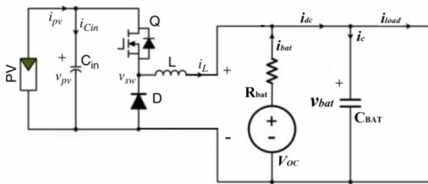
The SPV system equivalent circuit is illustrated in Figure 1. The PVG includes one PV array with nine PV modules. The current iload specifies all DC loads supplied by the battery and controlled by a DC-DC buck converter. The battery electrical circuit is designed by a voltage source VOC in series with a resistance Rbat, with an equivalent capacitor CBAT in parallel.
Figure 1. Equivalent circuit of the SPV system
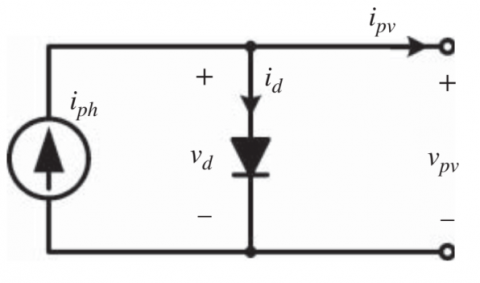
For reasons of simplicity, the photovoltaic cell is considered as an ideal current source providing a current Iph proportional to the incident light power, in parallel with a diode having the P-N junction. Therefore, the PV cell can be modelled by Figure 2, whose corresponding characteristics (Ipv-Vpv) are given in terms of cell temperature T and solar irradiance G according to the following equation [12]:
$i_{p v}=i_{p h}(G, \Delta T)-\underbrace{i_{s}(G, \Delta T)\left[e^{\left(\frac{q v_{p v}}{k T_{c} A_{n}}\right)}-1\right]}_{i_{d}(G, \Delta T)}$ (1)
The values of the constants, variables and model parameters of Eq. (1) are listed in Table 1.
Figure 2. Scheme of PV cell
Table 1. PV parameters
|
Components |
Rating values |
|
Irradiance at STC |
1000 W∕m2 |
|
Boltzmann constant |
K=1.38 × 10⁻²³ J/K |
|
Electron Charge |
1.6 × 10⁻¹⁹ C |
|
Diode ideality factor |
An = 1.6 |
|
PV cell temperature at STC |
298 K |
|
Thermal voltage of p-n junction at STC |
25.7 mV |
|
PV Cells number per module |
60 |
|
PV array configuration |
3 × 3 PV modules |
|
PV power at MPP and STC |
280 W / module |
|
PV voltage at MPP and STC |
31.67V |
|
PV current at MPP and STC |
8.84A |
|
PV open-circuit voltage at the STC |
38.97V |
|
PV short-circuit current at the STC |
9.41A |
|
Temperature coefficient on PV current |
0.04%/℃ |
|
Temperature coefficient on PV voltage |
-0.29%/℃ |
|
Irradiance coefficient on PV power |
-0.40%/℃ |
By combining NS identical cells in series, and NP cells in parallel, the resultant characteristics (IpvM-VpvM) of the PV module are given by relations (2) and (3):
$I_{p v M}=N_{S} I_{p v}$ (2)
$\mathrm{V}_{p v M}=N_{P} v_{p v}$ (3)
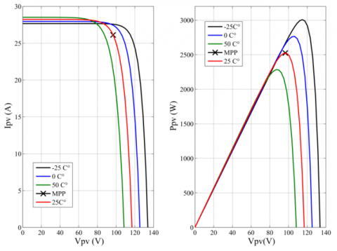
Figure 3. PV panel curves at various temperatures
Figure 4. PV panel curves under various irradiances
The curves in Figures 3 and 4 show the characteristics (I,V) and (I,P) of the PV panel under study, configured within three modules in series and three modules in parallel. the non-linear feature of each curve has a single optimal point MPP which will be the subject of the tracking algorithms studied during this paper.
The model of the battery given by Eq. (4) measures the instantaneous battery voltage vbat corresponding to the charge current ibat [12]:
$v_{b a t}=V_{O C}-R_{b a t} \cdot i_{b a t}$ (4)
To simulate the voltage source, we used the specific battery BK-10V10T, which is a Panasonic NiMH product. According to the available datasheets of this product, it is preferable to convert its discharge capacity Cdis into a state of charge (SOC), which is a parameter defining the battery voltage according to the following polynomial function [13]:
$V_{O C}=P_{5} S O C^{5}+P_{4} S O C^{4}+P_{3} S O C^{3}$$+P_{2} S O C^{2}+P_{1} S O C+P_{0}$ (5)
where, polynomial coefficients, P5, P4, P3, P2, P1, and P0 are reported in Table 2 [13].
Table 2. Polynomial constants of battery module BK-10V10T
|
Components |
Rating values |
|
P5 |
42.2942 |
|
P4 |
-98.3961 |
|
P3 |
88.7769 |
|
P2 |
-40.3893 |
|
P1 |
10.2942 |
|
P0 |
11.4802 |
We deduce then, the simulation block of the battery output voltage as a function of the current as given in Figure 5.
Figure 5. Simulink model of the battery
The equivalent circuit dynamics in Figure 1 linking the inductor current iL and the battery input current ibat, can be given by Eq. (6) and (7).
$i_{L}+i_{b a t}=C_{B A T} \frac{d v_{b a t}}{d t}+i_{\text {load }}$ (6)
$R_{b a t} C_{B A T} \frac{d i_{b a t}}{d t}+i_{b a t}=i_{\text {load }}-i_{L}$ (7)
We deduce from Eq. (6) and (7), the transfer function of Eq. (8).
$i_{b a t}(s)=\frac{i_{load}-i_{L}}{R_{b a t} \,\,C_{B A T}\,\, S+1}$ (8)
An effective control of the overall SPV system consists in judiciously controlling the duty cycle D of the converter by following a well-determined approach. For dynamic modelling, SPV output voltage is valued to be constant on continuous conduction mode (CCM). Based on the switching device conduction state Q, we differentiate two cases:
Q on-state Dynamics:
$L \frac{d i_{L}}{d t}=v_{p v}-v_{0}$ (9)
$C_{i n} \frac{d v_{p v}}{d t}=i_{p v}-i_{L}$ (10)
Q off-state Dynamics:
$L \frac{d i_{L}}{d t}=-v_{0}$ (11)
$C_{i n} \frac{d v_{p v}}{d t}=i_{p v}$ (12)
Due to the non-linearity of the output PV generator and the switching mode, it is appropriate to develop an averaged mathematical model to precisely control the system by neglecting fast switching dynamics. The Tayler expansion series appeared the main tool of local approximation of functions, allowing to linearize the differential equations associated with electrical circuits.
Using only the first-order approximation, the Taylor series of an infinitely differentiable function g(x), near a point of balance x0 is given by [14]:
$g(x) \approx g\left(x_{0}\right)+\left.\underbrace{\frac{d g(x)}{d x}}_{a_{1}}\right|_{x=x_{0}}\left(x-x_{0}\right)$ (13)
Under this approach, the differential equation x’=g(x) can be approximated for a disturbance $\tilde{x}=x-x_{0}$ by the following expression [14]:
$\frac{d({{x}_{0}}+\tilde{x})}{dt}\approx g({{x}_{0}})+{{a}_{1}}(\tilde{x})$ (14)
With, a1 is a constant parameter.
The final linear model is then derived as:
$\frac{d(\tilde{x})}{dt}\approx {{a}_{1}}(\tilde{x})$ (15)
By generalizing this approach to the multi-states and inputs systems, a nonlinear differential equation with two state variables x1 and x2 and one input I is given by:
$\left\{ \begin{matrix} \frac{d{{x}_{1}}}{dt}=g({{x}_{1}},{{x}_{2}},I) \\ \frac{d{{x}_{2}}}{dt}=g({{x}_{1}},{{x}_{2}},I) \\\end{matrix} \right.$ (16)
Using Eqns. (9) to (12), and based on the previous theoretical reasoning, the PV system dynamics can be expressed as:
$\frac{d{{i}_{L}}}{dt}=g({{i}_{L}},{{v}_{pv}},d)$ (17)
$\frac{d{{v}_{pv}}}{dt}=f({{i}_{L}},{{v}_{pv}},d)$ (18)
A linear model can be achieved at steady state using partial derivatives of Eqns. (17) and (18).
$\frac{d{{{\tilde{i}}}_{L}}}{dt}=\left. \frac{\partial g}{\partial {{v}_{pv}}} \right|{{\tilde{v}}_{pv}}+\left. \frac{\partial g}{\partial {{i}_{L}}} \right|{{\tilde{i}}_{L}}+\left. \frac{\partial g}{\partial d} \right|\tilde{d}$ (19)
$\frac{d{{{\tilde{v}}}_{pv}}}{dt}=\left. \frac{\partial f}{\partial {{v}_{pv}}} \right|{{\tilde{v}}_{pv}}+\left. \frac{\partial f}{\partial {{i}_{L}}} \right|{{\tilde{i}}_{L}}+\left. \frac{\partial f}{\partial d} \right|\tilde{d}$ (20)
where, $\tilde{d}, \tilde{i}_{L}$, and $\widetilde{v_{p v}}$ are steady state small signals of duty cycle d, current iL, and PV panel voltage Vpv that are considered constant in steady state.
By averaging the Eqns. (9) to (12), we get the nonlinear system defined by Eqns. (21) and (22):
$\frac{d{{i}_{L}}}{dt}=\underbrace{\frac{1}{L}\left[ d{{v}_{pv}}-{{v}_{O}} \right]}_{g({{v}_{pv}},d,{{i}_{L}})}$ (21)
$\frac{d{{v}_{pv}}}{dt}=\underbrace{\frac{1}{{{C}_{in}}}\left[ d{{i}_{pv}}-d{{i}_{L}} \right]}_{f({{v}_{pv}},d,{{i}_{L}})}$ (22)
Using the linearization procedure of Eqns. (19) and (20), a state space model can be expressed via Eqns. (21) and (22) under nominal operating conditions:
$\left[ \begin{matrix} \frac{d{{{\tilde{i}}}_{L}}}{dt} \\ \frac{d{{{\tilde{v}}}_{pv}}}{dt} \\\end{matrix} \right]=\left[ \begin{matrix} 0 & \frac{D}{L} \\ -\frac{D}{{{C}_{in}}} & \frac{1}{{{R}_{pv}}\,\,{{C}_{in}}} \\\end{matrix} \right]\left[ \begin{matrix} {{{\tilde{i}}}_{L}} \\ {{{\tilde{v}}}_{pv}} \\\end{matrix} \right]+\left[ \begin{matrix} \frac{{{v}_{pv}}}{L} \\ -\frac{{{i}_{L}}}{{{C}_{in}}} \\\end{matrix} \right]\tilde{d}$ (23)
By select d as the control variable, system dynamics can be designed by the following second order transfer function:
$\frac{{{{\tilde{v}}}_{pv}}(s)}{\tilde{d}(s)}=\frac{-\frac{{{i}_{L}}}{{{C}_{in}}}s-\frac{D{{v}_{pv}}}{L{{C}_{in}}}}{{{s}^{2}}-(\frac{1}{{{R}_{pv}}\,\,{{C}_{in}}})s+\frac{{{D}^{2}}}{L{{C}_{in}}}}$ (24)
The normalized form G0(s) of Eq. (24) is achieved by rearranging different terms:
${{G}_{0}}(s)=\frac{{{k}_{0}}(\beta s+1)}{{{s}^{2}}+2\xi {{\omega }_{n}}s+\omega _{n}^{2}}$ (25)
where, ξ is the damping factor and ωn is the natural undamped frequency. By analogy, we can easily determine the proper coefficients of Eq. (25). We suggest to control the system using simple PID controller with the following standard form:
$C(s)={{k}_{p}}+\frac{{{k}_{i}}}{s}+\frac{{{k}_{d}}}{\tau .s+1}$ (26)
PID parameters are shown in Table 3.
Table 3. PID parametres
|
Components |
values |
|
Kp |
-0.0017 |
|
Ki |
-8.4736 |
|
Kd |
- 6.8485x10⁻⁶ |
|
$\tau$ |
2.8745x10⁻⁴ |
In the literature, we can find different types of commands performing the PPM search. In this contribution, we will discuss three methods: Perturb and Observe (P&O); fuzzy logic controller; and Incremental conductance (Inc-Cond). To better understand these controls’ performances, we briefly recall their various principles below.
4.1 Perturb and Observe (P&O) method
The theory of P&O method is to disturb the VPV voltage of small breadth close to the initial value, to assess the resulting power variability PPV. Thus, it can be inferred that VPV voltage positive increment ensues in an increase of the PPV power, this implies that the operating point is located at the left of the PPM. The system will outstrip the PPM point if the power decreases. A similar reasoning can be made when the voltage decreases. Based on these findings governing the effect of voltage variation on the PPV(VPV) characteristics, it is convenient to locate the operating point regarding PPM point, and converge it with an appropriate command. Based on this principle and its related Eq. (27), the P&O flowchart is shown in Figure 6.
$\left\{ \begin{matrix} \begin{matrix} {} & \frac{dp}{dv}\succ 0 & \begin{matrix} \begin{matrix} if & \frac{\Delta I}{\Delta V}\succ -\frac{I}{V} \\\end{matrix} & {} \\\end{matrix} \\\end{matrix} \\ \begin{matrix} {} & \frac{dp}{dv}=0 & \begin{matrix} \begin{matrix} if & \frac{\Delta I}{\Delta V}=-\frac{I}{V} \\\end{matrix} & {} \\\end{matrix} \\\end{matrix} \\ \begin{matrix} {} & \frac{dp}{dv}\prec 0 & \begin{matrix} if & \frac{\Delta I}{\Delta V}\prec -\frac{I}{V} & {} \\\end{matrix} \\\end{matrix} \\\end{matrix} \right.$ (27)
Despite its precision and speed of reaction, P&O algorithm has some problems, as the oscillations around the PPM under typical operating conditions, and the deficient converging against sudden variations in the temperature and/or irradiance [15, 16].
Figure 6. Flowchart of P&O algorithm
4.2 Incremental Conductance (Inc-Cond) Technique
The MPPT command allows the search of the PPM operating point depending on the convergence of the conductance increment ΔG=ΔI/ΔV and conductance G=I/V in the following equation [17, 18]:
$\frac{dp}{dv}=V\frac{di}{dv}+1\approx V\frac{\Delta I}{\Delta V}+1$ (28)
Maximum power MPP is reached when the PV slope is null at MPP, negative in the right, and positive on the left as follows:
$\left\{ \begin{matrix} \begin{matrix} {} & \frac{dp}{dv}\succ 0 & \begin{matrix} \begin{matrix} if & \frac{I}{V}\succ -\frac{di}{dv} \\\end{matrix} & {} \\\end{matrix} \\\end{matrix} \\ \begin{matrix} {} & \frac{dp}{dv}=0 & \begin{matrix} \begin{matrix} if & \frac{I}{V}=-\frac{di}{dv} \\\end{matrix} & {} \\\end{matrix} \\\end{matrix} \\ \begin{matrix} {} & \frac{dp}{dv}\prec 0 & \begin{matrix} if & \frac{I}{V}\prec -\frac{di}{dv} & {} \\\end{matrix} \\\end{matrix} \\\end{matrix} \right.$ (29)
Figure 7. Flowchart of the Inc-Cond algorithm
Practically, like the P&O method, this technique has oscillations around the point MPP, because it is difficult to fulfil the condition dp/dv =0, the flowchart of the algorithm is presented in Figure 7.
4.3 Fuzzy logic control algorithm
The fuzzy logic concept is one of the important branches of artificial intelligence, which was introduced by Professor Lotfi Zadeh in 1965. Fuzzy logic controllers are appropriate of functioning with imprecise inputs; it is not necessary to have accurate parameters or precise mathematical model, manage nonlinearity and control a complicated system [19].
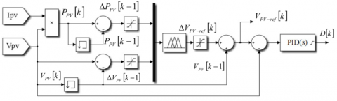
The fuzzy logic control is performed in three steps: fuzzification, inference, and Dufuzzification. The input variables adopted in this paper are the variation of the PVG power (ΔPPV) and photovoltaic voltage (ΔVPV), and the output variable is the variation of PV reference voltage (ΔVref) according to the equations [20]:
$\left\{ \begin{matrix} \Delta P=P(k)-P(k-1) \\ \Delta V=V(k)-V(k-1) \\ V{{(k)}_{ref}}=V(k-1)+\Delta {{V}_{ref}} \\\end{matrix} \right.$ (30)
where, k is the sampling time, P(k) is the actual PVG power, and V(k) is the corresponding instantaneous voltage.
During fuzzification, numeric input variables are converted within language variables that can take the following member function values (Table 4): NB (Negative Big), PB (Positive Big), NM (Negative Medium), PM (Positive Medium), NS (Negative Small), PS (Positive Small), ZE (Zero).
Table 4. Fuzzy rules
|
ΔVref |
ΔPPV |
|||||||
|
ΔVPV |
|
NB |
NM |
NS |
Z |
PS |
PM |
PB |
|
NB |
PB |
PB |
PM |
Z |
NM |
PB |
NB |
|
|
NM |
PB |
PM |
PS |
Z |
NS |
NM |
NB |
|
|
NS |
PM |
PS |
PS |
Z |
NS |
NS |
NM |
|
|
Z |
NB |
NM |
NS |
Z |
PS |
PM |
PB |
|
|
PS |
NM |
NS |
NS |
Z |
PS |
PS |
PM |
|
|
PM |
NB |
NM |
NS |
Z |
PS |
PM |
PB |
|
|
PB |
NB |
NB |
NM |
Z |
PM |
PB |
PB |
|
On the fuzzy logic MPPT structure of Figure 8, the PID downstream controller is used to rate the duty cycle D monitoring the converter.
Figure 8. Fuzzy logic MPPT structure
4.4 Integrating MPPT with battery-charge control
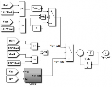
To avoid possible battery overload, the control strategy must simultaneously check both the MPPT and the charging cycle as shown in Figure 9. If the battery current or voltage reaches their load cycle limits, the PVG production shall be reduced by disabling the MPPT. Otherwise, the PVG operating point should be transferred in the open-circuit voltage. The battery DC link parameters are given in Table 5.
Table 5. Battery DC link parameters
|
Components |
Rating values |
|
Battery type |
NiMH |
|
Battery model |
BK-10V10T |
|
Battery pack voltage rating |
55 V |
|
Band of voltage limits |
54.45-55.45 V |
|
Nominal capacity |
90 Ah |
|
Nominal voltage of DC load |
48 V |
|
Acceptable voltage range of DC load |
42-56 V |
Figure 9. Integrating of MPPT and battery control
The overall simulation block of SPV system is shown in Figure 10.
Figure 10. Overarching model of simulation
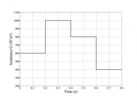
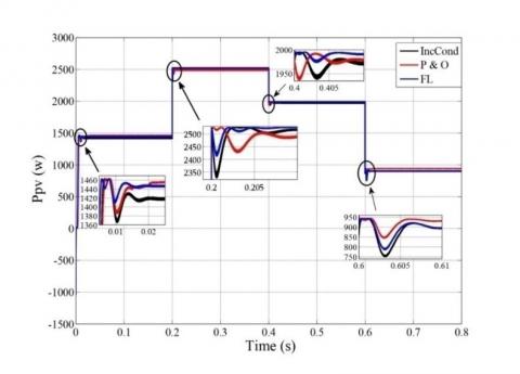
To validate the model and since the cadence of temperature change is relatively slow, we subject it to a fast variation of solar irradiance levels as shown in Figure 11, while maintaining the temperature at 25℃. Simulation results are illustrated in Figures 12 to 16. A steady rated load of 2.8A is simulated powered by the battery link. SPV output powers plotted in Figure 12 show that the operating point is regularly close to the MPP throughout the tracking phase, with more or less significant dissimilarity between the three methods. Fuzzy logic controller exhibits relatively better performances with very good dynamics compared to other strategies, in terms of speed tracking, MPPT tracking accuracy, especially at high irradiance levels.
Figure 11. Irradiance vs time
Figure 12. PVG power curves
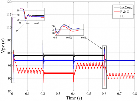
Figure 13. PVG terminal voltage curves
Figure 13 shows PVG terminal voltages for all methods. The operating point voltage monitoring process is activated when the battery voltage is between the lower limit VLo-lim and upper limit VUp-lim. In our case, it extends during the start-up period up to 0.2s and between 0.4s and 0.8s as shown in Figure 15. Unlike FLC and IncCond algorithms having good tracking behavior with fewer oscillations, the voltage ripple arising from the dynamic perturbation of the P & O technique is noticeable.
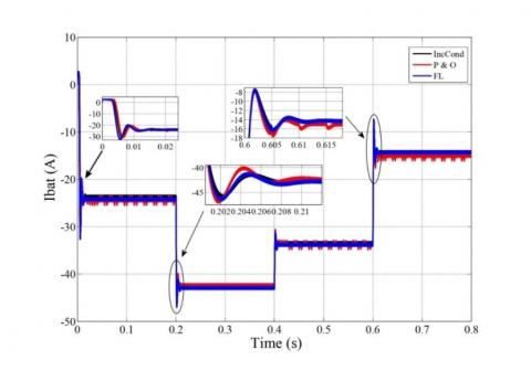
The battery voltages shown in the Figure 14 for all methods are well within the manufacturer’s tolerable limits VLo-lim and VUp-lim. In the time-bound range between 0.2s to 0.4s, where solar irradiance is more important, The PV output power significantly enhances, inducing an increase in the charging current as shown in Figure 15. Voltage reaches the upper limit with good quality, because the control strategy used disables the MPPT process. Outside of this interval, the battery voltage is even below the upper limit VUp-lim, and the MPPT remains active to inject more power into the battery link, which affects the voltage and current qualities, especially, that achieved by the P&O method.
The initial state of charge of the battery was set to be 80% as shown in Figure 16. The SOC progresses increasingly regarding the charging current, and since it is relatively low, the battery voltage is rather under the higher limit VUp-lim. Meanwhile, it is obvious that SOC is relatively faster with FC controller.
Figure 14. Battery voltage
Figure 15. Battery charging current
Figure 16. Battery state of charge
In this paper, a PID controller of a stand-alone photovoltaic system with battery charging was designed to control the battery charging process and track the maximum power point (MPP). Given the non-linear behavior of the PV system, a specific methodology based on Tayler’s expansion series is opted in this work, to derive a linear model used to analyze system dynamics and design the regulator. PID controller was applied with three different MPPT algorithms to enhance system performances, even under the rapid changes of the irradiance, and control the battery pack to correspond with its nominal voltage. A typical 2525W PV system was simulated in short term to pick up fast dynamics transitional details. Simulation results show good performances and prove SPV system effectiveness of design, modelling, and monitoring. Particularly, very good dynamics are achieved applying fuzzy logic controller compared to other strategies, in terms of speed tracking, MPPT tracking accuracy, voltage quality, and reducing transient fluctuations. Further, it is recommended to improve the switching time between the optimization phase and the battery control phase, in the case of significant variations in the climatic conditions, or the electrical load related to the system. This can be better assessed by working over a long simulation term.
|
G |
Solar irradiance, W/m2 |
|
IM |
Instant MPP current, A |
|
iph |
PV photon current, A |
|
ipv |
PV cell output current, A |
|
Id |
Diode current, A |
|
Iss |
Diode reverse-bias saturation current,A |
|
TC |
PV cell temperature, K |
|
VD |
Diode voltage, V |
|
VM |
Instant MPP voltage, V |
|
VOC |
PV open-circuit voltage, V |
|
VPV |
PV cell terminal voltage, V |
|
An |
dimensionless, diode ideality factor in SDM |
|
IMS |
PV current at MPP and STS, A |
|
Iph |
PV photon current at STC, A |
|
ISCS |
PV short-circuit current at the STC, A |
|
IS |
Diode reverse-bias saturation current, A |
|
PMPP |
PV power at MPP and STC, W |
|
VMS |
PV voltage at MPP and STC, V |
|
VOCS |
PV open-circuit voltage at STC, V |
[1] Xiao, W. (2017). Photovoltaic Power System: Modeling, Design, and Control. John Wiley & Sons. https://doi.org/10.1002/9781119280408
[2] Precup, R., Kamal, T., Hassan, S.Z. (2019). Solar photovoltaic power plants: Advanced control and optimization techniques. Springer. Singapore. https://doi.org/10.1007/978-981-13-6151-7
[3] Subudhi, B., Pradhan, R. (2012). A comparative study on maximum power point tracking techniques for photovoltaic power systems. IEEE Transactions on Sustainable Energy, 4(1): 89-98. https://doi.org/10.1109/TSTE.2012.2202294
[4] Dabra, V., Paliwal, K.K., Sharma, P., Kumar, N. (2017). Optimization of photovoltaic power system: A comparative study. Protection and Control of Modern Power Systems, 2(1): 1-11. https://doi.org/10.1186/s41601-017-0036-2
[5] Kotla, R.W., Yarlagadda, S.R. (2021). Comparative analysis of photovoltaic generating systems using particle swarm optimization and cuckoo search algorithms under partial shading conditions. Journal Européen des Systèmes Automatisés, 54(1): 27-33. https://doi.org/10.18280/jesa.540104
[6] Cheng, P.C., Peng, B.R., Liu, Y.H., Cheng, Y.S., Huang, J.W. (2015). Optimization of a fuzzy-logic-control-based MPPT algorithm using the particle swarm optimization technique. Energies, 8(6): 5338-5360. https://doi.org/10.3390/en8065338
[7] Liu, C.L., Chen, J.H., Liu, Y.H., Yang, Z.Z. (2014). An asymmetrical fuzzy-logic-control-based MPPT algorithm for photovoltaic systems. Energies, 7(4): 2177-2193. https://doi.org/10.3390/en7042177
[8] Li, X., Wen, H., Hu, Y., Du, Y., Yang, Y. (2020). A comparative study on photovoltaic MPPT algorithms under EN50530 dynamic test procedure. IEEE Transactions on Power Electronics, 36(4): 4153-4168. https://doi.org/10.1109/TPEL.2020.3024211
[9] Tang, S., Sun, Y., Chen, Y., Zhao, Y., Yang, Y., Szeto, W. (2017). An enhanced MPPT method combining fractional-order and fuzzy logic control. IEEE Journal of Photovoltaics, 7(2): 640-650. https://doi.org/10.1109/JPHOTOV.2017.2649600
[10] Fapi, C.B.N., Wira, P., Kamta, M., Colicchio, B. (2020). Voltage regulation control with adaptive fuzzy logic for a stand-alone photovoltaic system. European Journal of Electrical Engineering, 22(2): 145-152. https://doi.org/10.18280/ejee.220208
[11] Altaş, I.H. (2017). Fuzzy logic control in energy systems with design applications in MATLAB/Simulink. IET. ISBN: 9781785611070.
[12] Messaoud, M., Haddi, B. (2021). Optimum parametric identification of a stand-alone photovoltaic system with battery storage and optimization controller using averaging approach. Journal Européen des Systèmes Automatisés, 54(1): 63-71. https://doi.org/10.18280/jesa.540108
[13] Panasonic industry Nickel hybrid Battery. (2020). https://industrial.panasonic.com/content/data/BT/docs/edbd/ni_mh/IntroductionofNickelMetalHydrideBattery_Web_20200203.pdf.
[14] Drazin, P.G., Drazin, P.D. (1992). Nonlinear Systems. Cambridge University Press. http://doi.org/10.1017/CBO9781139172455
[15] De Brito, M.A., Sampaio, L.P., Luigi, G., Melo, G.A., Canesin, C.A. (2011). Comparative analysis of MPPT techniques for PV applications. In 2011 International Conference on Clean Electrical Power (ICCEP), pp. 99-104. https://doi.org/10.1109/ICCEP.2011.6036361
[16] Rekioua, D., Matagne, E. (2012). Optimization of photovoltaic power systems: Modelization, simulation and control. Springer Science & Business Media. https://doi.org/10.1007/978-1-4471-2403-0
[17] Lorenzini, G., Kamarposhti, M.A., Solyman, A.A.A. (2021). Maximum power point tracking in the photovoltaic module using incremental conductance algorithm with variable step length. Journal Européen des Systèmes Automatisés, 54(3): 395-402. https://doi.org/10.18280/jesa.540302
[18] Khadidja, S., Mountassar, M., M'hamed, B. (2017). Comparative study of incremental conductance and perturb & observe MPPT methods for photovoltaic system. In 2017 International Conference on Green Energy Conversion Systems (GECS), pp. 1-6. https://doi.org/10.1109/GECS.2017.8066230
[19] Ross, T.J. (2010). Fuzzy Logic with Engineering Applications. John Wiley & Sons. https://doi.org/10.1002/9781119994374
[20] Yilmaz, U., Kircay, A., Borekci, S. (2018). PV system fuzzy logic MPPT method and PI control as a charge controller. Renewable and Sustainable Energy Reviews, 81: 994-1001. https://doi.org/10.1016/j.rser.2017.08.048