Imane Ghlib* | Youcef Messlem | Zakaria Chedjara
© 2022 IIETA. This article is published by IIETA and is licensed under the CC BY 4.0 license (http://creativecommons.org/licenses/by/4.0/).
OPEN ACCESS
This article develops a new observer to achieve highly speed estimation for induction motor control. Its principle consists of estimating flux and speed separately, by using linear Luenberger as flux observer and intelligent PI controller as rotor speed estimator. Considering that is generally challenging to established proper PI parameters, the ADALINE algorithm is integrated as a trainable module to automatically calculate the KP and the KI gains in each iteration during all operation induction motor. This algorithm helps to search on the one hand the best regulation of the controller in real-time, taking into account the objectives to achieve (an accurate estimation) and the respect constraints (heavy calculation). On the other hand, it makes it possible to improve the adaptive Luenberger estimation problem in the unobservable zone (low speed). The experimental comparison of the observers demonstrates the visible improvement of the enhanced observer. It can converge to real speed in a short time with less static and transient error.
ADALINE, artificial neural network, induction motor, intelligent controller, Luenberger, sensorless control
Sensorless speed control of three-phase Induction Motor (IM) allows systems to be installed easily in many applications avoiding the fragility and the high cost of mechanical speed sensors [1].
However, several numbers of important research have been published about sensor algorithms among them, the state observers.
They consist of modelling the induction motor by dynamic mathematical equations [2]. There are two classes of observers [3]. The first class: stochastic observers who are designed to eliminate measured signals’ noises. Kalman filter represents the optimal stochastic observer [4, 5], where its main problem is the cost of computationally is more intensive, as long as, the second of deterministic observers class neglect the noise [6] (Luenberger, MRAS …).
The MRAS (Model Reference Adaptive System) consists to estimate rotor flux and rotor speed separately. That's means, it uses Luenberger as a current and flux observer. These last are injected into the adaptive mechanism and compared with a measured current to calculate the rotor speed.
Intensive research effort has been focused on using PI controllers as an adaptation scheme. The simple structure of the PI regulator and the reduced cost of its realization lead to be used in 80% of industry applications [7, 8]. However, obviously and basically the determination of the proportional and integrator parameter (PI) is not optimal. Usually, most of the time these parameters are selected by the classic "try and error" method. that is to say, during the synthesis of the regulator, the values are being varied in each test so that the estimation errors are gradually being eliminated during the successive performances. In addition, these parameters remain fixed throughout the operation of the motor. which makes this observer not robust for internal and external changes (speed reversal, load charge….).
For this reason, artificial intelligence such as; genetic algorithms, fuzzy logic, artificial neural networks are introduced to enhance these kinds of observers [9-14], ... Previous studies have only been carried out in theory, because they are limited with algorithm complexity and the computing load. Furthermore, most of these studies have suffered from poorly developed in real-time.
In this paper, to overcome the previously cited drawbacks of the existing observers, an ADALINE (ADAptive LInear NEuron) algorithm [15, 16] is proposed. Its main advantages are that it is quick and simple to implement. Moreover, in parallel to other neural schemes that used multi-layer feed-forward [17-19], the ADALINE avoids delaying caused by calculation load.
That's why it has been had selected rather than the other techniques.
It is now well confirmed from a variety of studies in electrical engineering that, this algorithm proves its effectiveness in different fields such as the estimate and compensate for harmonics from an AC line [20], minimization the undesirable torque ripple for permanent magnet motor drive [21], and Identification of parameters of induction motor at standstill state [22, 23].
A new application of ADALINE is presented in this work, it is motivated by the desire to obtain improvement speed estimation, that uses an adaptive mechanism based on online learning, to replace the conventional PI controller.
However, adaptive linear neurons compute the proportional and integrator gains from the estimated model and measured currents.
The remainder of the paper is ordered as follows: in section 2, a description of direct field-oriented control of IM. Section 3 describes Neural MRAS for induction motor. Section 4 investigates the experimental results of Neural Luenberger in comparison with classical adaptive. Finally, section 5 gives some concluding remarks.
The principle of the vector control of the induction motor consists of adjusting the flux independently of the torque as DC motor.
- The flux is adjusted by acting only on the Isd component.
- The torque is regulated via the quadratic component Isq.
The application of this command is allowed by applying the decoupling technique. So, the objective is to direct the flux to have only one component on the direct axis. We will therefore have to cancel the quadratic flux.
$\left\{ \begin{matrix} {{\varphi }_{rd}}={{\varphi }_{r}} \\ {{\varphi }_{rq}}=0 \\ \end{matrix} \right.$ (1)
φrd is the direct axis components of rotor flux.
φrq is the quadratic axis components of rotor flux.
The dynamic equations of stator current components isd and isq, direct rotor flux and electromagnetic torque will then be reduced to:
$\left\{ \begin{matrix} \frac{d{{i}_{sd}}}{dt}=\frac{1}{\sigma {{L}_{s}}}\left( -\left( {{R}_{s}}+{{(\frac{{{M}_{sr}}}{{{L}_{r}}})}^{2}}{{R}_{r}} \right){{i}_{sd}}+\sigma L{}_{s}{{\omega }_{s}}{{i}_{sq}}+\frac{{{M}_{sr}}{{R}_{r}}}{L_{r}^{2}}{{\phi }_{r}}+{{V}_{sd}} \right) \\ \frac{d{{i}_{sq}}}{dt}=\frac{1}{\sigma {{L}_{s}}}\left( -\left( {{R}_{s}}+{{(\frac{{{M}_{sr}}}{{{L}_{r}}})}^{2}}{{R}_{r}} \right)iq-\sigma L{}_{s}{{\omega }_{s}}{{i}_{sd}}+\frac{{{M}_{sr}}{{R}_{r}}}{L_{r}^{{}}}{{\phi }_{r}}{{\omega }_{r}}+{{V}_{sq}} \right) \\ \frac{d{{\phi }_{rd}}}{dt}=\frac{p{{M}_{sr}}}{{{L}_{r}}}{{i}_{sd}}-\frac{{{R}_{r}}}{{{L}_{r}}}{{\phi }_{r}} \\ {{T}_{e}}=\frac{p{{M}_{sr}}}{{{L}_{r}}}{{i}_{sq}}{{\phi }_{r}} \\ \end{matrix} \right.$ (2)
Figure 1. Bloc of induction motor vector control
Figure 1 describes a direct field-oriented control scheme. In which two PI (Proportional-integrator) controllers are used for currents control, while The IP (integrator-proportional) speed regulator is a combination of two loops of an I regulator and a P regulator that have been mounted in cascade. It is important to mention that the lack of a speed sensor can cause à trouble for the control of the motor. Furthermore, the flux can’t be measured for economic reasons, but its knowledge is essential to guarantee a high level of performance. Since the whole variables of the state vector (flux and speed) are not measured often, they must be estimated using an observer. This is sensorless control. without affecting the stability of the closed-loop, the synthesis of the observer must respond the requirements of vector control. Furthermore, the accuracy of state estimation is no longer for itself, but the complete system control of the state is the overall goal. The observer is an essential part of the order, i.e., the observer error should be minimized as much as possible to guarantee the stability of all closed-loop.
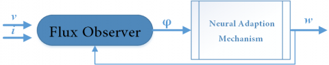
Generally, for nonlinear systems (induction motor), an adaptive observer is used to separate the estimation of the rotor speed from all the other variables (stator currents and rotor flux). This technique provides a good solution for the IM non-linearity problem. Figure 2 shows the principle of the neural adaptive observer. In this structure, there are two cascading loops. First, the state vector variables are estimated by a linear flux observer which considers the speed to be a known parameter. the latter is calculated in the second loop by an adaptive mechanism. The purpose of this paper is to explore a new adaptation scheme to improve the MRAS observer.
Figure 2. Principal of adaptive observer
3.1 System model
In order to reduce the size of the state vector, and consequently the complexity of the model, the hypothesis of decoupling of the mechanical mode (the rotor speed) with regard to the electric modes (stator currents) and magnetic (rotor flux) has been applied. Considering speed as a known parameter, the space-state of the induction motor will be a linear system.
The matrix representation that will allow the synthesize of the observer will therefore be the following:
$\begin{aligned} \frac{d}{d t} x &=A(x)+B(u) \\ &=\left(\begin{array}{cc}A_{11} & A_{12} \\ A_{21} & A_{22}\end{array}\right)\left(\begin{array}{l}i_{s} \\ \varphi_{r}\end{array}\right)+\left(\begin{array}{l}B_{1} \\ 0\end{array}\right) \end{aligned}$ (3)
with:
$A_{11}=-\left\{\mathrm{Rs} /(\sigma \mathrm{Ls})+(1-\sigma) /\left(\sigma \tau_{r}\right)\right\} \mathrm{I}=a_{r 11} I$
$A_{12}=M s r /(\sigma L s L r)\left\{\left(1 / \tau_{\mathrm{r}}\right) \mathrm{I}-\mathrm{W}_{\mathrm{r}} \mathrm{J}\right\}=a_{r 12} I+a_{i 12} J$
$A_{21}=\left(\mathrm{Msr} / \tau_{\mathrm{r}}\right) \mathrm{I}=a_{r 21} I$
$A_{22}=-\left(1 / \tau_{r}\right) I+\omega_{r} J=a_{r 22} I+a_{i 22} J$
$B_{1}=(1 / \sigma L s) I=b_{1} I$
$I=\left(\begin{array}{ll}1 & 0 \\ 0 & 1\end{array}\right)$ and $J=\left(\begin{array}{cc}0 & -1 \\ 1 & 0\end{array}\right)$
where, $x=\left[\begin{array}{llll}i_{s d} & i_{s q} & \varphi_{r d} & \varphi_{r q}\end{array}\right]^{T}$, and y=[isd isq]T.
3.2 Flux observer
One of the major issues of the direct field-oriented vector control of the induction motor is that the rotor flux is not directly measurable, and therefore its estimation from known variables (stator currents and voltages) is indispensable. The flux observer is given in ref. [13] for the system (3) can be described by the following equations:
$\frac{d}{dt}\hat{X}=A\hat{X}+BU+G({{\hat{i}}_{s}}-{{i}_{s}})$ (4)
where, the symbol ^ is used to describe the estimated variables, The gain matrix G is determined so that observer (4) can be stable.
$G=-\left[ \begin{align} & {{g}_{1}}{{I}_{1}}+{{g}_{2}}{{J}_{2}} \\ & {{g}_{3}}{{I}_{1}}+{{g}_{4}}{{J}_{2}} \\ \end{align} \right]$
To ensure a good estimate of the rotor flux, it must choose the observation gain G such that (A-GC) is asymptotically stable, i.e.: the eigenvalues of (A-GC) matrix must have a negative real part.
$\left\{ \begin{align} & {{g}_{1}}=(k-1)({{a}_{r11}}+{{a}_{r22}}) \\ & {{g}_{2}}=(k-1){{a}_{i22}} \\ & {{g}_{3}}=({{k}^{2}}-1)(c{{a}_{r11}}+{{a}_{r21}})-c(k-1)({{a}_{r11}}+{{a}_{r22}}) \\ & {{g}_{4}}=-c(k-1){{a}_{i22}} \\ \end{align} \right.$
Because the induction motor itself is stable in typical operation, then the adaptive observer will be also stable.
3.3 Speed estimation
The deterministic observer MRAS presented in ref. [13] uses a PI adaptation mechanism to estimate rotor speed. The adaptation stability has been proved by the means of the estimation error. It has been derived by the Lyapunov theory by choosing an adequate candidate function
$\begin{aligned} e &=X-\hat{X} \\ \Delta A=\hat{A}-A &=\left[\begin{array}{cc}0 & -\Delta \omega_{r} J / c \\ 0 & \Delta \omega_{r} J / c\end{array}\right] \end{aligned}$ (5)
where, $c=\left(\sigma L_{s} L_{r}\right) / M_{s r}$ and $\Delta \omega_{r}=\hat{\omega}_{r}-\omega_{r}$.
Lyapunov function candidate:
$V={{e}^{T}}e+{{({{\hat{\omega }}_{r}}-{{\omega }_{r}})}^{2}}/\lambda $ (6)
where, λ is a positive constant.
The derivate of V in time:
$\frac{d}{d t} V=e^{T}\left\{(A+G C)^{T}+(A+G C)\right\} e-\left(2 \Delta \omega_{r}\left(e_{i d s} \hat{\varphi}_{d r}-e_{i q s} \hat{\varphi}_{q r}\right)\right) / c+2 \Delta \omega_{r} \frac{d}{d t} \widehat{\omega}_{r} / \lambda$ (7)
The following speed estimation equation is obtained, by the equating the second and the third term of the Eq. (7).
$\frac{d}{dt}{{\hat{\omega }}_{r}}=\lambda ({{e}_{ids}}{{\hat{\varphi }}_{dr}}-{{e}_{iqs}}{{\hat{\varphi }}_{qr}})/c$ (8)
The speed generation is carried out using the following equation:
${{\hat{\omega }}_{r}}={{K}_{p}}({{e}_{ids}}{{\hat{\varphi }}_{qr}}-{{e}_{iqs}}{{\hat{\varphi }}_{dr}})+{{K}_{i}}\int{({{e}_{ids}}{{{\hat{\varphi }}}_{qr}}-{{e}_{iqs}}{{{\hat{\varphi }}}_{dr}})dt}$ (9)
This PI controller is designed to calculate rotor speed with the following transfer function:
${{C}_{PI}}(S)={{K}_{p}}+{{K}_{i}}\frac{1}{s}$ (10)
The PI controller is a required module for the adaptive observers. The setting of PI controller parameters can be considered as an optimization problem or it is a question of finding the optimal solution of the controller gains. Several analytical techniques have been proposed to calculate the adapter components meanwhile they presented a challenge for the adaptive observer. The gains [Kp, Ki] are often selected by a classical method “try and error”. It is about performing as plenty of tests as necessary and adjusting various attempts until acceptable gains are established. It is iterative, it takes time and generally, the gains founded by that classical strategy are not precise to be included in the training of high performances. Besides, these adaptive mechanisms are unsatisfactory because they can be adversely affected by certain conditions (Since these gains are fixed).
For these reasons, considering that is generally challenging to set proper PI parameters, the ADALINE algorithm is integrated as a learning module to automatically calculate the pair of parameters [Kp, Ki].
3.4 The ADALINE neural network
Learning ADALINE ADAptive LInear NEurons is made online and is based on minimizing the error by performing a calculation so that the ADALINE weights converge to optimal coefficients (LMS algorithm) [20].
An artificial ADALINE is a network that has just an input and only one output, during the experiment the ADALINE adjusts its weights immediately after including the input vector [15].
Figure 3. ADALINE learning rule topology
It is a very simple structure with input vector x(k) is multiplied with suitable weight factors w(k), and the obtained results are summed up and introduced to the output vector y(k) (Figure 3).
${{y}_{k}}=\sum\limits_{i=1}^{n}{x{{(i)}_{k}}{{w}_{k}}=x_{i}^{T}{{w}_{k}}}$ (11)
${{w}_{k+1}}={{w}_{k}}+\Delta w$ (12)
3.5 ADALINE for adaptive scheme speed estimation
The synthesis of the conventional PI controller was done according to the proceeding of KUBOTA [13]. Its major problem is in the method used to calculate the pair of gains [Kp, Ki]. They are obtained by test and error. those gains are unadjustable. However, they clearly are not valid for overcoming long-term problems in different situations.
Figure 4. Block diagram of neural adaptive neural observer
The main contribution of this paper is to resolve the problem of tuning these two adaptation parameters using the neural network algorithm of ADALINE (Figure 4). they are learned online in each iteration with two weights. w0 is for auto-tuning the Kp (proportional gain). And a second weight w1 is used for learning the integral parameter [8].
The ADALINE algorithm calculates the intelligent gains [Kp, Ki] in each iteration for guaranteeing the convergence of the estimated speed to the real one regardless of the system conditions. This learning rule is making possible the simplification of the intelligent controller, reduces the cost of calculation, and at the same time improves the observer's stability.
Our study consists in verifying experimentally ADALINE in the adaptation mechanism of the observer developed. It is noted that this approach is original. However, for reasons of obvious comparison, the conventional regulators are kept and the values obtained by the observer are introduced into the control loop instead of the measured value.
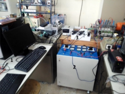
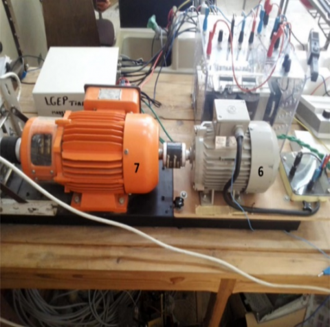
The test bench (Figure 5) contains an actuator composed of an induction motor associated with a synchronous generator (Figure 6), a power supply consisting of an autotransformer (2), a SEMIKRON type inverter (4), and a Dspace1104 control card (5).
The system is controlled in real-time via the Control Desk platform of the Dspace card.
Figure 5. Test bench
Figure 6. Induction motor (6) associated with a synchronous generator (7)
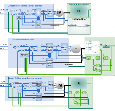
Figure 7. Block diagram of sensorless control of induction motor
The objective of the experimental tests is to verify the effectiveness of the algorithm of ADALINE in real-time for the observation. For this purpose, comparisons are made between the conventional method and the proposed method. The results obtained are represented by the catch recording under Control Desk. The entire block diagram of the sensorless control system can be seen in the Figure 7.
In Table 1, the motor parameters are collected.
Table 1. Parameters of the IM
|
Parameters |
Values |
Units |
|
Rs |
5.6 |
Ω |
|
Rr |
5.6081 |
Ω |
|
Ls |
0.5310 |
H |
|
Lr |
0.6164 |
H |
|
Lm |
0.5496 |
H |
|
P |
1 |
- |
|
Rated speed |
2780 |
Rpm |
|
Rated power |
750 |
W |
Experimental verification for observers (conventional and advanced) has been taking place in two stages:
•The first test consists to verify the speed direction under two kinds of conditions; reversal of the direction of rotation of the induction motor and varying load charge.
•The second is to test observers in a band of medium and under a low speed.
4.1 Speed reversal
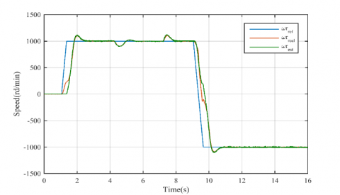
Figures 8-9 show the motor responses (red curves) to speed reference (the blue curves) from 0 rpm (state of rest) to +1000 rpm (transient state). Then it is fixed in a static regime with applying a load torque. Next, the sense of rotation of the reference is inversed to -1000 rpm in a very short time (0,6 s).
Note that green curves in both figures represent estimated speed.
Comparing the two results (Figure 8 with Figure 9), it can be seen that the results obtained by the observer improved by ADALINE are less sensitive to the impact of variations in speed and load torque than with the classic. (Figure 10).
Both observers have the same flux estimator gain and are presented in the same closed-loop control but they have different adaptive mechanisms. To achieve an accurate speed estimation ADALINE is used because it presents an advanced learning rule that adapts its parameters automatically. As illustrated in Figure 10, the estimated speeds are close to their real values is remarked, where the errors tend to zero.
Figure 8. Real and estimated speeds using Neural Luenberger
Figure 9. Real and estimated speeds using classical Luenberger
(a) Neural Luenberger
(b) Classical Luenberger
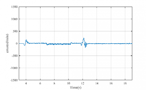
Figure 10. The estimation error
(a)
(b)
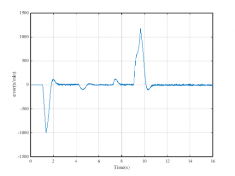
Figure 11. The pursuit error (a) neural Luenberger (b) classical Luenberger
The Figures 11 (a) and (b) represent the pursuit error for the real speed and the reference wrreal-wrref, noted that the state estimate is obtained via a state observer and the estimate state $\hat{x}$ is used in vector control. With the PI regulator, the transient error is greater than 1000 rpm. However, it is minimised under ADALINE observer, when the load torque is supplied, the overshoot error is reduced.
4.2 Medium speed
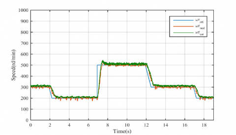
To test the stability of the intelligent algorithm, we apply average set point speeds of 500 rpm, 300 rpm and 200 rpm, Figures 12-13 expose the measured and estimated speed.
In Figure 13, the difference between the measured speed and the estimated speed is significant and clearly observed when the speed is reduced to the value of 200 rpm.
From Figure 12, it is clear that the estimated rotor speed perfectly follows the speed of the motor. These results show the effectiveness of the learning algorithm when it is used in the adaptation mechanism in order to realize an observer. Note also, the elimination of static errors in the speed even at the reference of 200rpm is achieved. The values thus estimated showed their stabilities all along and during the operation. The learning phenomenon of ADALINE is well estimated less than the second.
Figure 12. Real and estimated speeds using Neural Luenberger
Figure 13. Real and estimated speeds using classical Luenberger
A new adaptive mechanism for MRAS observer was developed in this paper, which estimates speed and flux for sensorless vector control of induction machine. PI parameters of the adaption mechanism are learned online with the ADALINE network. It means that the gains of the regulator are self-tuned in each iteration during all the operations of the system. So that the speed estimation converges to the real value.
According to the experimental results obtained the application of ADALINE type artificial intelligence makes it possible to achieve these objectives: the speed of response and the robustness with regard to the disturbances of the load, which makes it possible to obtain an accurate estimation. It is characterized by its ease of implementation and its short calculation time. It can be concluded that this applied strategy allows a visible improvement of the vector control and the estimation of the speed.
|
Vsd, Vsq |
The d-q axis components of stator voltage |
|
ids, iqs |
The d-q axis components of stator current |
|
φrd, φrq |
The d-q axis components of rotor flux |
|
Rr, Rs |
The rotor and stator resistances |
|
Lr, Ls Msr |
he rotor, stator and mutual inductances |
|
$\omega_{s}$ |
The synchronous speed in rad/s |
|
$\omega_{r}$ |
The rotor speed (mechanical) in rad/s |
|
$\sigma$ |
The leakage coefficient |
[1] Xu, D., Wang, B., Zhang, G., Wang, G., Yu, Y. (2018). A review of sensorless control methods for AC motor drives. CES Transactions on Electrical Machines and Systems, 2(1): 104-115. https://doi.org/10.23919/TEMS.2018.8326456
[2] Dawson, D.M., Hu, J., Brug, T.C. (2019). Nonlinear Control of Electric Machinery. Routledge. https://doi.org/10.1201/9780203745632
[3] Demir, R., Barut, M. (2018). Novel hybrid estimator based on model reference adaptive system and extended Kalman filter for speed-sensorless induction motor control. Transactions of the Institute of Measurement and Control, 40(13): 3884-3898. https://doi.org/10.1177/0142331217734631
[4] Maybeck, P.S. (1982). Stochastic Models, Estimation, and Control. Academic Press.
[5] Zerdali, E. (2018). Adaptive extended Kalman filter for speed-sensorless control of induction motors. IEEE Transactions on Energy Conversion, 34(2): 789-800. https://doi.org/10.1109/TEC.2018.2866383
[6] Berrezzek, F., Benheniche, A. (2021). Backstepping based nonlinear sensorless control of induction motor system. J. Eur. Systèmes Autom., 54(3): 495-502. https://doi.org/10.18280/jesa.540313
[7] Dasari, M., Mani, V. (2019). Simulation and analysis of PI and NN tuned pi controllers for transformer based three-phase multi-level inverter with MC-PWM techniques. J. Eur. Systèmes Autom., 52(6): 587-598. https://doi.org/10.18280/jesa.520606
[8] Hassan, H., Azar, A.T., Tembi, T.D., Khatthy, T., Sosa, A. (2018). Design and implementation of fuzzy PID controller into multi agent smart library system prototype. in The International Conference on Advanced Machine Learning Technologies and Applications (AMLTA2018), pp. 127-137. https://doi.org/10.1007/978-3-319-74690-6_13
[9] Bennassar, A., Abbou, A., Akherraz, M., Barara, M. (2014). A new sensorless control design of induction motor based on backstepping sliding mode approach. International Review on Modelling and Simulations, 7(1): 35-42. https://doi.org/10.15866/iremos.v7i1.247
[10] Fekik, A., Denoun, H., Azar, A.T., et al. (2018). Artificial neural network for PWM rectifier direct power control and DC voltage control. In Advances in System Dynamics and Control, pp. 286-316. https://doi.org/10.4018/978-1-5225-4077-9.ch010
[11] Gadoue, S.M., Giaouris, D., Finch, J.W. (2009). MRAS sensorless vector control of an induction motor using new sliding-mode and fuzzy-logic adaptation mechanisms. IEEE Transactions on Energy Conversion, 25(2): 394-402. https://doi.org/10.1109/TEC.2009.2036445
[12] Ghariani, M., Hachicha, M.R., Ltifi, A., Bensalah, I., Ayadi, M., Neji, R. (2011). Sliding mode control and neuro-fuzzy network observer for induction motor in EVs applications. International Journal of Electric and Hybrid Vehicles, 3(1): 20-46. https://doi.org/10.1504/IJEHV.2011.040471
[13] Kubota, H., Matsuse, K., Nakano, T. (1993). DSP-based speed adaptive flux observer of induction motor. IEEE Transactions on Industry Applications, 29(2): 344-348. https://doi.org/10.1109/IAS.1991.178183
[14] Zhu, Q., Azar, A.T. (2015). Complex system modelling and control through intelligent soft computations (Vol. 319). London, UK: Springer. https://doi.org/10.1007/978-3-319-12883-2
[15] Widrow, B., Winter, R.G., Baxter, R.A. (1988). Layered neural nets for pattern recognition. IEEE Transactions on Acoustics, Speech, and Signal Processing, 36(7): 1109-1118. https://doi.org/10.1109/29.1638
[16] Widrow, B., Lehr, M.A. (1990). 30 years of adaptive neural networks: perceptron, madaline, and backpropagation. Proceedings of the IEEE, 78(9): 1415-1442. https://doi.org/10.1109/5.58323
[17] Cirrincione, M., Pucci, M., Cirrincione, G., Capolino, G.A. (2007). Sensorless control of induction machines by a new neural algorithm: The TLS EXIN neuron. IEEE Transactions on Industrial Electronics, 54(1): 127-149. https://doi.org/10.1109/TIE.2006.888774
[18] Gadoue, S.M., Giaouris, D., Finch, J.W. (2009). Sensorless control of induction motor drives at very low and zero speeds using neural network flux observers. IEEE Transactions on Industrial Electronics, 56(8): 3029-3039. https://doi.org/10.1109/TIE.2009.2024665.
[19] Abbas, H.A., Zegnini, B., Belkheiri, M. (2015). Neural network-based adaptive control for induction motors. In 2015 IEEE 12th International Multi-Conference on Systems, Signals & Devices (SSD15), pp. 1-6. https://doi.org/10.1109/SSD.2015.7348180
[20] Abdeslam, D.O., Wira, P., Mercklé, J., Flieller, D., Chapuis, Y.A. (2007). A unified artificial neural network architecture for active power filters. IEEE Transactions on Industrial Electronics, 54(1): 61-76. https://doi.org/10.1109/TIE.2006.888758
[21] Flieller, D., Nguyen, N.K., Wira, P., Sturtzer, G., Abdeslam, D.O., Mercklé, J. (2013). A self-learning solution for torque ripple reduction for nonsinusoidal permanent-magnet motor drives based on artificial neural networks. IEEE Transactions on Industrial Electronics, 61(2): 655-666. https://doi.org/10.1109/TIE.2013.2257136
[22] Bechouche, A., Sediki, H., Abdeslam, D.O., Haddad, S. (2011). A novel method for identifying parameters of induction motors at standstill using ADALINE. IEEE Transactions on Energy Conversion, 27(1): 105-116. https://doi.org/10.1109/TEC.2011.2175393
[23] Imane, G., Youcef, M., Abdelmadjid, G., Zakaria, C. (2017). Neural adaptive Kalman filter for sensorless vector control of induction motor. International Journal of Power Electronics and Drive Systems, 8(4): 1841‑1851. https://doi.org/10.11591/ijpeds.v8.i4.pp%p