Rafik Euldji* | Noureddine Batel | Redha Rebhi | Noureddine Kaid | Chutarat Tearnbucha | Weerawat Sudsutad | Giulio Lorenzini | Hijaz Ahmad | Houari Ameur | Younes Menni
© 2022 IIETA. This article is published by IIETA and is licensed under the CC BY 4.0 license (http://creativecommons.org/licenses/by/4.0/).
OPEN ACCESS
A design of an optimal backstepping fractional order proportional integral derivative (FOPID) controller for handling the trajectory tracking problem of wheeled mobile robots (WMR) is examined in this study. Tuning parameters is a challenging task, to overcome this issue a hybrid meta-heuristic optimization algorithm has been utilized. This evolutionary technique is known as the hybrid whale grey wolf optimizer (HWGO), which benefits from the performances of the two traditional algorithms, the whale optimizer algorithm (WOA) and the grey wolf optimizer (GWO), to obtain the most suitable solution. The efficiency of the HWGO algorithm is compared against those of the original algorithms WOA, GWO, the particle swarm optimizer (PSO), and the hybrid particle swarm grey wolf optimizer (HPSOGWO). The simulation results in MATLAB–Simulink environment revealed the highest efficiency of the suggested HWGO technique compared to the other methods in terms of settling and rise time, overshoot, as well as steady-state error. Finally, a star trajectory is made to illustrate the capability of the mentioned controller.
optimization algorithms for robotics, wheeled mobile robot, trajectory tracking, back-stepping controller, fractional order proportional integral derivative controller, meta-heuristic, particle swarm optimizer, grey wolf optimizer, hybrid particle swarm grey wolf optimizer, hybrid whale grey wolf optimizer
Nowadays, wheeled mobile robots (WMRs) are well-known for their ability to be used in both civilian and military tasks such as reconnaissance, agriculture, rescue, space exploration, surveillance, combat, materials transportation, etc. [1-9]. Recently, problems related to trajectory tracking of WMR still taking the remarkable attention of many researchers [10]. However, many research papers focusing only on enhancing the performance of the kinematic controller [11-13].
The reason behind choosing the previously mentioned controller is that the dynamic controller's design is more complex than the kinematic one since the dynamics depend on the robot parameters such as the moment of inertia, mass, frictions [14]. Defining the dynamics of robot vehicles is needed in some applications, such as high-speed motions and heavy transportation. For that purpose, a sliding mode dynamic controller was proposed by Esmaeili et al. [15, 16], an online physical parameters adaptation of the robot dynamics is proposed by Shanmugavel et al. [17], using adaptive neural network controller to handle unmodeled dynamics by Fierro et al. [18, 19], while Das & Kar [20] investigated an online training using an adaptive fuzzy logic controller to learn the complete dynamics.
Typically, the PID control technique (traditional proportional integral derivative) is still employed in various industrial processes. This is mainly because of the simple structure and eases of design and implementation. When significant robustness and transient efficiency are required, the control effect is limited. To handle this kind of problems, the fractional order proportional integral derivative (FOPID) controller is adopted for this purpose. It is obtained by the combination of fractional calculus and the traditional PID controller, which introduces two new parameters λ and μ (the integral and derivative fractional-order, respectively) to the classic PID control. Those two added parameters have increased the performance and the robustness of the controller; several papers demonstrate the high efficiency and performance of FOPID controller compared to classic PID controller [21, 22].
In the last decade, the popularity of FOPID control has widely increased and attracted more attention in many engineering areas, including robotics engineering [1, 10, 23-27]. Tuning the five parameters (Kp, Kd, KI, λ and μ) of the FOPID controller is a challenging task compared to conventional PID control. Also, because WMR is a high coupled nonlinear system, taking into account some particular constraints such as the gain margin and sensitivity conditions [28].
Therefore, obtaining the optimal combination of these parameters can only be reached by using powerful optimizations methods. Meta-heuristic algorithms have proved their ability in turning the FOPID controller parameters and improving the controller’s performance in various studies. We distingue, particle swarm optimizer (PSO) [10, 28, 29], whale optimizer (WOA), grey wolf optimizer (GWO), and sine-cosine algorithm (SCA) [30-32].
So far, there is no optimization technique that could out-perform the rest in every aspect; researchers are always obligate to develop new algorithms with the aim to receive better results. One of the standard solutions is to realize various hybrid algorithms to combine the powerful points of the approaches [33]. Like, using the hybrid particle swarm grey wolf optimizer (HPSOGWO) [34] and the hybrid whale grey wolf optimizer (HWGO) [35].
The objective of this research is to design a back-stepping fractional order PID to control the WMR motion. Two blocs of the FOPID controller are used in the internal loop as a dynamic controller to guarantee that the linear and angular speeds of robot mobile follow their reference values. In addition, a back-stepping controller located in the external loop for controlling the kinematics, in the context of designing a robust controller, a powerful optimization technique is needed for the parameters tuning, as a consequence, a comparative study of different nature-inspired algorithms has been invested in selecting the best optimum method. In the same context, this paper proposes the HWGO algorithms to solve this kind of problem. The simulation results in MATLAB highlight the over efficiency of the HWGO algorithm compared to those of PSO, GWO, HPSOGWO, and WOA approaches. The performance criteria used for the minimization of the error are obtained using the cost functions, namely integral square error ISE. The study is presented as follows: The wheeled mobile robot is modeled and presented in Section 2. The controller design and strategy are described in Section 3. The algorithms used for tuning parameters, as well as the simulation findings and analysis are summarized in Sections 4 and 5, respectively.
2.1 Modeling the wheeled mobile robot
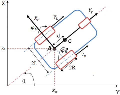
The WMR in Figure 1 contains two pairs of DC motors with driving wheels of radius R, where φL and φR are the left and right rotating angles of wheels, respectively. θ is the robot orientation and L is the width of the robot body. At the distance d from the mind-point A, where (Xa, Ya) is the coordinate of A in the inertial frame (X,Y), and the coordinates of any point in the robot frame are defined by (Xr, Yr).
Three steps are necessary to obtain the mathematical model of the robot mobile: kinematic modeling, dynamic modeling, and actuator modeling, which are defined as follows:
2.1.1 Kinematic model
This section aims to define a relationship between the linear and angular speeds of the mechanical systems without taking into account the forces affecting the motion [10, 11]. The linear speed of each driving wheel is:
$\left\{\begin{array}{l}\mathcal{v}_{R}=R \dot{\varphi}_{R} \\ \mathcal{v}_{L}=R \dot{\varphi}_{R}\end{array}\right.$ (1)
Figure 1. Schematic design of the WMR
The linear and angular velocities of the WMR are given by Eqns. (2) and (3), respectively:
$v=\frac{v_{R}+v_{L}}{2}=R \frac{\left(\dot{\varphi}_{R}+\dot{\varphi}_{L}\right)}{2}$ (2)
$\omega=\frac{v_{R}-v_{L}}{2 L}=R \frac{\left(\dot{\varphi}_{R}-\dot{\varphi}_{L}\right)}{2 L}$ (3)
The kinematic constraint can express by the following equations [36]:
No slip constraint:
$-\dot{x}_{a} \sin \theta+\dot{y}_{a} \cos \theta=0$ (4)
Pur rolling constraint:
$\dot{x}_{a} \cos \theta+\dot{y}_{a} \sin \theta+L \dot{\theta}=R \dot{\varphi}_{R}$
$\dot{x}_{a} \cos \theta+\dot{y}_{a} \sin \theta-L \dot{\theta}=R \dot{\varphi}_{L}$ (5)
The three constraint equations are:
$\Lambda(q) \dot{q}=0$ (6)
where:
$(q)=\left[\begin{array}{ccccc}-\sin \theta & \cos \theta & 0 & 0 & 0 \\ \cos \theta & \sin \theta & L & -R & 0 \\ \cos \theta & \sin \theta & -L & 0 & -R\end{array}\right]$ (7)
and
$\dot{q}=\left[\dot{x}_{a} \dot{Y}_{a} \dot{\theta}_{R} \dot{\varphi}_{L}\right]^{T}$ (8)
So, the kinematic model obtained is:
$\left[\begin{array}{c}\dot{x}_{a} \\ \dot{y}_{a} \\ \dot{\theta} \\ \dot{\varphi}_{R} \\ \dot{\varphi}_{L}\end{array}\right]=\left[\begin{array}{cc}\cos \theta & 0 \\ \sin \theta & 0 \\ 0 & 1 \\ \frac{1}{R} & \frac{-L}{R} \\ \frac{1}{R} & \frac{-L}{R}\end{array}\right]\left[\begin{array}{c}v \\ \omega\end{array}\right]=\frac{1}{2}\left[\begin{array}{cc}\cos \theta & 0 \\ \sin \theta & 0 \\ 0 & 1 \\ \frac{1}{R} & \frac{-L}{R} \\ \frac{1}{R} & \frac{-L}{R}\end{array}\right]\left[\begin{array}{c}\dot{\varphi}_{R} \\ \dot{\varphi}_{L}\end{array}\right]$ (9)
which may be written as:
$\dot{q}=S(q)_{\eta}$ (10)
where, $n=\left[\begin{array}{c}\dot{\varphi}_{\mathrm{R}} \\ \dot{\varphi}_{\mathrm{L}}\end{array}\right]$ is the vector of the angular velocities of two wheels.
2.1.2 Dynamical model
The purpose of dynamic modeling is to take into account all the different forces and energies that affect the mechanical system motion. The motion equation of the WMRs is given by [36, 37]:
$\begin{aligned} M(q) \ddot{q}+V(q, \dot{q}) \dot{q}+F(\dot{q})+G(q)+\tau_{d} \\=& B(q) \tau-\Lambda^{T}(q)^{\lambda} \end{aligned}$ (11)
For simulation purposes and control, Eq. (11) should be transformed into an alternative form, using the kinematic model (10):
$S^{T}(q) \Lambda^{T}(q)=0$ (12)
The new matrices are express as follows:
$\left\{\begin{array}{c}\bar{M}(q)=S^{T}(q) M(q) S(q) \\ \bar{V}=S^{T}(q) M(q) \dot{S}(q)+S^{T}(q) V(q, \dot{q}) S(q) \\ \bar{B}=S^{T}(q) B(q)\end{array}\right.$ (13)
The reduced form of the dynamic equations is expressed as:
$\{\bar{M}(q) \dot{\eta}+\bar{V}(q, \dot{q}) \eta=\bar{B}(q) \tau$ (14)
where,
$\bar{M}(q)=\left[\begin{array}{cc}I_{w}+\frac{R^{2}}{4 L^{2}}\left(m L^{2}+I\right) & \frac{R^{2}}{4 L^{2}}\left(m L^{2}-I\right) \\ \frac{R^{2}}{4 L^{2}}\left(m L^{2}-I\right) & I_{w}+\frac{R^{2}}{4 L^{2}}\left(m L^{2}+I\right)\end{array}\right]$ (14a)
and
$\begin{aligned} \bar{V}(q, \dot{q})=& {\left[\begin{array}{cc}0 & \frac{R^{2}}{2 L} m_{c} d \dot{\theta} \\ -\frac{R^{2}}{2 L} m_{c} d \dot{\theta} & 0\end{array}\right] }, \\ \bar{B}(q)=\left[\begin{array}{ll}1 & 0 \\ 0 & 1\end{array}\right] \end{aligned}$ (14b)
Eq. (14) may be rewritten in a compact form:
$\left\{\begin{array}{c}\left(m+\frac{2 I_{w}}{R^{2}}\right) \dot{v}-m_{c} d \omega^{2}=\frac{1}{R}\left(\tau_{R}+\tau_{L}\right) \\ \left(I+\frac{2 L^{2}}{R^{2}} I_{w}\right) \omega+m_{c} d \omega v=\frac{L}{R}\left(\tau_{R}-\tau_{L}\right)\end{array}\right.$ (15)
where, $m=m_{c}+2 m_{w}$ is the total mass of the robot, and $I=I_{c}+m_{c} d^{2}+2 m_{w} L^{2}+2 I_{m}$ represents the total equivalent inertia.
2.1.3 Actuator modeling
Two pairs of dc motors are considered as actuators for producing the torque to control the inputs for driving the wheels of the WMR as presented by Figure 2. The dynamic model of the actuators can be represented as [38]:
$\left\{\begin{aligned} v_{a}=R_{a} i_{a}(t) &+L_{a} \frac{d i_{a}(t)}{d t}+e_{a}(t) \\ e_{a}(t) &=K_{b} \omega_{m}(t) \\ \tau_{m}=j \frac{d w_{m}(t)}{d t} &+f w_{m}(t)+K_{t} i_{a}(t) \\ \tau &=N \tau_{m} \end{aligned}\right.$ (16)
where, ia is the armature current, (Ra, La) is the resistance and inductance of the armature winding, respectively, ea is the back emf, ωm is the rotor angular speed, τm is the motor torque, (Kt, Kb) are the torque constant and back emf constant, respectively, N is the gear ratio, and τ is the output torque applied to the wheel Since the robot motors are mechanically coupled to wheels through the gears.
Figure 2. Equivalent electrical schema of the dc motor
Therefore, each dc motor will have:
$\left\{\begin{aligned} \omega_{m R}=N \dot{\varphi}_{w R} & & \text { and } \tau_{R}=N \tau_{m R} \\ \omega_{m L}=N \dot{\varphi}_{w L} & & \text { and } \tau_{L}=N \tau_{m L} \end{aligned}\right.$ (17)
For the two motors, the dynamic model is expressed as:
$\begin{cases}\frac{1}{\left(R+L_{a} P\right)}\left(e_{a r}-K_{b} N \dot{\varphi}_{w R}\right)=i_{R} & \text { with } \tau_{R}=N k_{t} i_{R} \\ \frac{1}{\left(R+L_{a} P\right)}\left(e_{a l}-K_{b} N \dot{\varphi}_{w L}\right)=i_{L} & \text { with } \tau_{L}=N k_{t} i_{L}\end{cases}$ (18)
The robot physical parameters are provided in Table 1 [38].
Table 1. Physical parameter of the robot
|
Parameters |
Value and Unit |
|
Distance between two wheels, 2 L |
0.75 m |
|
Distance of point Pc from point Po, D |
0.3 m |
|
Driving wheels radius, R |
0.15 m |
|
Mass of the mobile robot without the driving wheels and DC motors, mc |
30 kg |
|
Mass of each driving wheel (with actuator), mw |
1 kg |
|
Moment of inertia of the mobile robot about the vertical axis through the center of mass, Ic |
15.625 kg∙m2 |
|
Moment of inertia of each driving wheel with a motor about the Wheel axis, Iw |
0.005 kg∙m2 |
|
Moment of inertia of each driving wheel with a motor about the Wheel diameter, Im |
0.0025 kg∙m2 |
|
Armature winding resistance, Ra |
1.6 Ω |
|
Armature winding inductance, La |
0.048 H |
|
Torque constant, Kt |
0.2613 N.m/A |
|
Back emf constant, Kb |
0.19 rad/s |
|
Gear ratio, N |
62.55 |
2.2 Controller design and strategy
Figure 3 presents the schematic design of the control strategy based on the dynamic and kinematic of the wheeled mobile robot. The trajectory generator produces the reference coordinate x, y and θ, a back-stepping kinematic controller is located in the external loop, here the controller experiences the difference between the reference data received from the bloc trajectory generator and actual value from the robot then generate his own angular and linear speeds that are sent into the internal loop where two blocs of FOPID controller are used as a dynamic controller. Here the two FOPID controllers yield their own signals of angular and linear speeds based on the reference values obtained from the kinematic controller.
Figure 3. Control scheme of WMR
2.2.1 Kinematic controller design
One of the goals here is to realize path tracking. The back-stepping technique has been widely used and is well known as a stable tracking control rule which makes it adopted for this purpose [11, 14]. The controller structure is highlighted in Figure 3, where the input error and velocity vector (vc) are:
$\left[\begin{array}{l}e_{x} \\ e_{y} \\ e_{\theta}\end{array}\right]=\left[\begin{array}{ccc}\cos \theta & \sin \theta & 0 \\ -\sin \theta & \cos \theta & 0 \\ 0 & 0 & 1\end{array}\right]\left[\begin{array}{cc}X_{r}- & X \\ Y_{r}- & Y \\ \theta_{r}- & \theta\end{array}\right]=T_{e} e_{r}$ (19)
$v_{c}=\left[\begin{array}{c}v_{r} \cos \left(e_{\theta}\right)+k_{x} e_{x} \\ w_{r}+k_{y} v_{r} e_{y}+k_{\theta} v_{r} \sin \left(e_{\theta}\right)\end{array}\right\rfloor$ (20)
where, kx, ky and kθ are the tuning parameters.
2.2.2 Dynamic controller description
The fractional proportional integral derivative FOPID was first proposed in 1999 by Podlubny [39]. Introducing the two new fractional components λ and μ to the classic PID controller under the name of Fractional integrator and differentiator respectively, the operator of non-integer-order is provided in Eq. (21) [40].
$D_{n}^{t}= \begin{cases}\frac{d^{n}}{d t^{n}} & n>0 \\ 1 & n=0 \\ \int_{t}^{a} d t^{n} & n<0\end{cases}$ (21)
where, a and t are the lower limit and upper limit of the process and $n \in \mathbb{R}$ the constant integral differential operator.
The fractional calculus has three main definitions Riemann Liouville (RL), Grünwald Letnikov (GL), and Caputo. The most common definition utilized in engineering applications is the Caputo method [30, 40] given in Eq. (22).
$D_{n}^{t} f(t)=\frac{1}{\Gamma(\alpha-n)} \int_{a}^{t} \frac{f^{n}(\tau)}{(t-\tau)^{n-\alpha+1}} d \tau$ (22)
for $n-1 \leq n \leq \alpha$ . The term sα doesn’t have an analytical solution, but it has a fractional order, which is hard to implement. Therefore, numerical solutions such as Oustaloup approximation are adopted [40].
$s^{\alpha} \approx K \prod_{n=-N}^{N} \frac{1+\frac{s}{\omega_{z, n}}}{1+\frac{s}{\omega_{p, n}}} \quad \alpha>0$ (23)
where, N is the number of poles/zeros. Figure 4 presents the parallel structure of the FOPID controller block diagram. Where E(S) distinguishes for the input and errors (E(S) and U(S)).
Figure 4. Block diagram of fractional order
Figure 5. Generalized FOPID controller
The representation of the transfer function for the Fractional Order PID (FOPID) in the time domain (Eq. (24)) and the transfer function corresponds to the fractional order in the Laplace domain (Eq. (25)).
$u(t)=K_{p} e(t)+k_{i} D_{t}^{-\lambda} e(t)+K_{d} D_{t}^{\mu} e(t)$ (24)
$C(s)=\frac{U(s)}{E(s)}=K_{p}+\frac{K_{i}}{s^{\lambda}}+K_{d} S^{\mu}$ (25)
where, Kp, Ki and Kd are proportional, integral and derivative gains constants, respectively, $\lambda$ and $\mu$ are factional order of the integral and derivative term. All type of the classic PID may be obtained by taking $(\lambda, \mu)=\{(1,1),(1,0),(0,1),(0,0)\}$, as shown in Figure 5.
2.2.3 Tuning parameters for FOPID
The WMR block diagram for tuning parameters of the Two FOPID controllers is highlighted in Figure 6. The first controller receives the difference between the reference and actual velocity from the right wheel as an input where the desired velocity is constant: Ur =1 m/s.
Figure 6. Bloc diagram for parameters tuning
The second controller in the left wheel experiences the difference between the actual and desired orientations as input. Where the reference angle was represented by a constant value: θr = 0.785 rad. The following Eq. (26) represent the relation between the input voltage of the right and left DC actuators, respectively UR, UL with the outputs of the first and second controller, respectively UV, Uθ:
$\left\{\begin{array}{l}U_{R}=\frac{U_{V}+U_{\theta}}{2} \\ U_{L}=\frac{U_{V}-U_{\theta}}{2}\end{array}\right.$ (26)
The cost function used in the study is the integral square error (ISE) which is demonstrated by Eq. (27):
$I S E=\left(\int_{0}^{\infty}\left[e_{v}(t)\right]^{2} d t+\int_{0}^{\infty}\left[e_{\theta}(t)\right]^{2} d t\right)$ (27)
where:
$\left\{\begin{array}{l}e_{v}=U_{r}-U_{m} \\ e_{\theta}=\theta_{r}-\theta_{m}\end{array}\right.$ (28)
Ur is the desired velocity, Um the actual velocity, ev the velocity error, θr the desired orientation, θm the measured orientation, and eθ is the orientation error. The optimization algorithms used to tune the parameters (Kp, KI, Kd, λ, µ) are described in the next section.
2.3 Meta-heuristic algorithms
2.3.1 Particle swarm optimization (PSO)
In this method and for each iteration, all of the particles in the swarm update their positions with the use of the following equations [34, 41]:
$\begin{aligned} V_{i}^{k+1}=w V_{i}^{k}+C_{1} & R_{1}\left(p_{i}^{k}+x_{i}^{k}\right) \\ &+C_{2} R_{2}\left(g b e s t_{i}+x_{i}^{k}\right) \end{aligned}$ (29)
$X_{i}^{k+1}=X_{i}^{k}+V_{i}^{k+1}$ (30)
Here, R1 and R2 are random numbers in the range [0, 1]. i refer to the particle in the swarm. k is the iteration step carried out, while w is the inertia weight parameter. The coefficients C1 and C2 are the optimization parameters, X: position vector, and $p_{i}^{k}$: best position information achieved by the ith particle, gbest $_{i}$: best position information available in the swarm [33].
2.3.2 Grey wolf optimizer (GWO)
The mathematical models of GWO consist of social hierarchy, enriching prey, search for prey, attacking prey, and hunting [42-44]. Social hierarchy: The leader of wolves is called alpha $(\alpha)$, Beta $(\beta)$ and delta $(\delta)$ are the second and third levels in the group, respectively.
$d=\left|c \cdot x_{p}(n)-x(n)\right|$ (31)
$(n+1)=x_{p}(n)-a \cdot d$ (32)
where, xp: position vector of the prey, n: current iteration, and x: position vector of a grey wolf. The vectors a and c are mathematically formulated as follows:
$\vec{a}_{(.)}=2 \vec{l} \cdot \vec{r}_{1}-\vec{l}$ (33)
$\vec{c}_{(.)}=2 \cdot \vec{r}_{2}$ (34)
where, r1 and r2 are random numbers in [0, 1]. The following equations for hunting are used:
$\left\{\begin{array}{l}\vec{d}_{\alpha}=\left|\vec{c}_{1} \cdot \vec{x}_{\alpha}-\vec{x}\right| \\ \vec{d}_{\beta}=\left|\vec{c}_{2} \cdot \vec{x}_{\beta}-\vec{x}\right| \\ \vec{d}_{\delta}=\left|\vec{c}_{3} \cdot \vec{x}_{\delta}-\vec{x}\right|\end{array}\right.$ (35a)
$\left\{\begin{array}{l}\vec{x}_{1}=\vec{x}_{\alpha}-\vec{a}_{1} \cdot\left(\vec{d}_{\alpha}\right) \\ \vec{x}_{2}=\vec{x}_{\beta}-\vec{a}_{2} \cdot\left(\vec{d}_{\beta}\right) \\ \vec{x}_{3}=\vec{x}_{\delta}-\vec{a}_{3} \cdot\left(\vec{d}_{\delta}\right)\end{array}\right.$ (35b)
$x(n+1)=\frac{\vec{x}_{1}+\vec{x}_{2}+\vec{x}_{3}}{3}$ (35c)
2.3.3 Hybrid PSO-GWO algorithm
HPSOGWO is the hybridize Particle Swarm Optimization with the Grey Wolf Optimizer algorithm that uses the functionalities of both variants to enhance exploitation in PSO and GWO and to generated both variants’ strength [34].
In this algorithm, the position of the first three agents is updated in the search space using Eq. (34). The control of the grey wolf exploration and exploitation is conducted with the inertia constant. Using the following modified equations:
$\begin{aligned} \vec{d}_{\alpha} &=\left|\vec{c}_{1} \cdot \vec{x}_{\alpha}-\omega * \vec{x}\right| \\ \vec{d}_{\beta} &=\left|\vec{c}_{1} \cdot \vec{x}_{\beta}-\omega * \vec{x}\right| \\ \vec{d}_{\delta} &=\left|\vec{c}_{1} \cdot \vec{x}_{\delta}-\omega * \vec{x}\right| \end{aligned}$ (36)
The following equation is for combining the variants of PSO and GWO:
$v_{i}^{k+1}=\omega *\left(\begin{array}{c}v_{i}^{k}+c_{1} r_{1}\left(x_{1}-x_{1}^{k}\right)+c_{2} r_{2}\left(x_{2}-x_{i}^{k}\right) \\ +c_{3} r_{3}\left(x_{3}-x_{i}^{k}\right)\end{array}\right)$
$x_{i}^{k+1}=x_{i}^{k}+v_{i}^{k+1}$ (37)
2.3.4 Whale optimization algorithm
This Algorithm consists of three stages [45-47]:
Bubble-net attacking method:
Using the bubble-net strategy, the humpback whales attack the prey. This is shown in the following two methods [45]:
$\vec{X}(n+1)=\vec{D}^{\prime} \cdot e^{b v} \cdot \cos (2 \pi v)+\vec{X}^{*}(n)$ (38)
$\vec{D}^{\prime}=\left|\vec{X}^{*}(n)-\overrightarrow{X(n)}\right|$ (39)
A probability of 50% to choose either a shrinking mechanism or a helical path down below the mathematical formula:
$\vec{X}(n+1)$
$=\left\{\begin{array}{l}\vec{X}^{*}(n)-\vec{A} \cdot \vec{D} \text { if } p<0.5 \\ \vec{D}^{\prime} \cdot e^{b v} \cdot \cos (2 \pi v)+\vec{X}^{*}(n) \text { if } p>0.5\end{array}\right.$ (40)
where, p is a random number in [0, 1].
Search for prey:
The humpback whales search randomly for prey. Exploitation phase fellow those rules [45]:
$\vec{D}=\left|\vec{C} \cdot \vec{X}_{\text {rand }}-\vec{X}\right|$ (41)
$\vec{X}(n+1)=\vec{X}_{\text {rand }}-\vec{A} \cdot \vec{D}$ (42)
2.3.5 Hybrid WOA-GWO algorithm
The HWGO algorithm aims to enhance the efficiency of the WOA algorithm by applying the leadership hierarchy of GWO. The next step is to apply the outcome to the WOA attacking strategy. The HWGO selected the three best candidate solutions: the 1st, 2nd, and 3rd levels in the group are alpha (a), beta (b), and delta (d).
The mathematical model for updating the position of whales using the leadership hierarchy of GWO during optimization is given as:
$\left\{\begin{array}{l}\vec{D}_{\alpha}^{\prime}=\left|\vec{X}_{\alpha}(n)-\vec{X}\right| \\ \vec{D}_{\beta}^{\prime}=\left|\vec{X}_{\beta}(n)-\vec{X}\right| \\ \vec{D}_{\delta}^{\prime}=\left|\vec{X}_{\delta}(n)-\vec{X}\right|\end{array}\right.$ (43)
$\left\{\left\{\begin{array}{l}\vec{X}_{1}(n)=\vec{X}_{\alpha}(n)+\vec{D}_{\alpha} \cdot e^{b v} \cdot \cos (2 \pi v) \\ \vec{X}_{2}(n)=\vec{X}_{\beta}(n)+\vec{D}_{\beta} \cdot e^{b v} \cdot \cos (2 \pi v) \\ \vec{X}_{3}(n)=\vec{X}_{\delta}(n)+\vec{D}_{\delta} \cdot e^{b v} \cdot \cos (2 \pi v)\end{array}\right.\right.$ (44)
$\left\{\vec{X}(n+1)=\frac{\vec{X}_{1}+\vec{X}_{2}+\vec{X}_{3}}{3}\right.$ (45)
This investigation adopted the use of various analyses such as convergence curve, the step response of linear velocity and orientation, and trajectory tracking in order to validate the performance and robustness of the suggested HWGO algorithm. In comparison to four optimization algorithms under the name of PSO, GWO, WOA, and HPSOGWO.
All simulation experiments of this study were performed on a PC independently, which had the following configuration: operating system, 64-bit Windows 10; CPU, Intel Core i5-4200 2.30 GHz, and simulation software, MATLAB R2019. To measure the robustness of the compared meta-heuristics in solving this problem we run more than 30 simulation experiments for each algorithm. Moreover, in order to study the convergence behavior of the algorithms, the maximum number iterations and the population size are set to 100 and 20, respectively.
3.1 Convergence curve of the algorithms
Figure 7 presents the convergence curve of the five selected optimizations algorithms. That’s proved the over-performance of the HWGO algorithm.
The obtained value of ISE for all algorithms used in the study is shown in Table 2. From Figure 7 and Table 2, it quite obvious that the PSO fells easy in local minimum, with a cost value (0.0504) compare to GWO that has obtained a better object function value (0.0477). The HPSOGWO could solve the problem by avoiding the local minimum related to PSO, and could reach a better precision than the GWO (0.0464). The WOA optimizer also as the PSO optimizer fells in the local minimum with the worst ISE value obtained (0.0533).
Figure 7. Convergence curve of five algorithms
Table 2. ISE values of the five algorithms
|
Algorithms |
PSO |
GWO |
HPSOGWO |
WOA |
HWGO |
|
ISE |
0.0504 |
0.0477 |
0.0464 |
0.0533 |
0.0452 |
However, this algorithm takes the smaller number of iterations (need only 10 iteration) compare to the previous mentioned approached. Lastly, the proposed HWGO algorithm that benefited from the rapidity of the WOA algorithm, and the precision of the GWO algorithm, could obtain the best cost value (0.0452). In summary, the HWGO algorithm has the lowest ISE amount with the highest rapidity in terms of convergence. It is noted that the algorithm only took 50 iterations to obtain the best optimal values.
3.2 Step response performance of speed controller
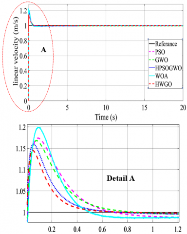
Figure 8 presents the comparative findings for velocity step responses that were designed with various techniques. As illustrated, the HWGO is characterized by a significant time response, as mentioned below.
Figure 8. Comparison of velocity step response for all algorithms
Table 3 shows the gain details of the FOPID1 controller, for the speed control of the WMR, for all chosen algorithms. While Table 4 shows the characteristics obtained in the time domain.
From Figure 8, and Tables 3 and 4, we can say that the best overshoot belongs to HWGO followed by HPSOGWO, GWO, PSO, and WOA by an overshoot of 14.514%, 16.211%, 16.689%, 17.366%, and 19.982%, respectively. The algorithms can classify from worst rise time to the best rise time as follows: PSO (0.0034s), GWO (0.0032s), HPSOGWO (0.0031s), WOA (0.0027s), and HWGO (0.0026s). Based on the settling time the algorithm can be classified as follows: PSO (0.4944s), GWO (0.4924s), WOA (0.3994s), HPSOGWO (0.3655s), and HWGO (0.3168s).
Table 3. The tuned gain details of FOPID1 Controller for all algorithms
|
Methods |
FOPID 1 for speed control |
||||
|
$K_{p}$ |
$K_{i}$ |
$K_{d}$ |
λ |
µ |
|
|
PSO |
400 |
100 |
100 |
0.96 |
0.66 |
|
GWO |
500 |
10.975 |
100 |
0.96 |
0.66 |
|
HPSOGWO |
500 |
99.69 |
100 |
0.11 |
0.65 |
|
WOA |
500 |
100 |
28.15 |
0.87 |
0.94 |
|
HWGO |
500 |
145 |
149 |
0.10 |
0.56 |
Table 4. Performance characteristic for FOPID1
|
Methods |
FOPID 1 for speed control |
||||
|
$t_{r}$ |
Mp% |
Peak |
$t_{p}$ |
$t_{s}$ |
|
|
PSO |
0.0034 |
17.366 |
1.1737 |
0.0890 |
0.4944 |
|
GWO |
0.0032 |
16.689 |
1.1669 |
0.0761 |
0.4924 |
|
HPSOGWO |
0.0031 |
16.211 |
1.1621 |
0.0509 |
0.3655 |
|
WOA |
0.0027 |
19.982 |
1.1998 |
0.0926 |
0.3994 |
|
HWGO |
0.0026 |
14.514 |
1.1451 |
0.0479 |
0.3168 |
3.3 Step response performance of angle controller
Figure 9 presents the comparative findings for angle step responses that were designed by applying the five optimization techniques. As illustrated, the HWGO has a significant time response.
Table 5 reveals the gain details of the FOPID2 controller for the orientation control of the WMR selected. In contrast, the comparative results of transient response are highlighted in Table 6.
From Figure 9, Tables 5 and 6, we can say that the best overshoot belongs to HWGO followed by GWO, HPSOGWO, WOA, and PSO by an overshoot of 0.8464%, 1.6377%, 2.3653%, 3.2358%, and 3.8347%, respectively.
The algorithms can classify from worst rise time to the best rise time as follows: GWO (0.5235s), WOA (0.4033s), HPSOGWO (0.4017s), PSO (0.3994s), and HWGO (0.225s). Based on the settling time the algorithm can be classified as follows: HPSOGWO (4.9513s), PSO (1.9409s), WOA (1.4563s), GWO (0.9705s), and HWGO (0.4914s).
Figure 9. Comparison of step response for the orientation
Table 5. The tuned main parameters of FOPID2 controller for all algorithms
|
Methods |
FOPID 2 for Angle control |
||||
|
$K_{p}$ |
$K_{i}$ |
$K_{d}$ |
λ |
µ |
|
|
PSO |
1 |
100 |
69.55 |
0.1 |
0.96 |
|
GWO |
1.21 |
57.22 |
74.18 |
0.15 |
0.96 |
|
HPSOGWO |
67.9 |
6.52 |
75.17 |
0.74 |
0.96 |
|
WOA |
93.48 |
3.17 |
63.46 |
0.60 |
0.96 |
|
HWGO |
63.97 |
26.4 |
81.95 |
0.36 |
0.95 |
Table 6. Performance characteristic for FOPID2
|
Methods |
FOPID 2 for speed control |
||||
|
$t_{r}$ |
Mp% |
Peak |
$t_{p}$ |
$t_{s}$ |
|
|
PSO |
0.3994 |
3.8347 |
0.8151 |
1.0770 |
1.9409 |
|
GWO |
0.5235 |
1.6377 |
0.7979 |
2.6191 |
0.9705 |
|
HPSOGWO |
0.4017 |
2.3653 |
0.8036 |
3.2517 |
4.9513 |
|
WOA |
0.4033 |
3.2358 |
0.8104 |
0.9832 |
1.4563 |
|
HWGO |
0.2825 |
0.8464 |
0.7916 |
2.2696 |
0.4914 |
In summary, the lowest amounts of peak percentage, overshoot (Mp%), rise time (tr for 10% → 90%), and settling time (ts for ±2% tolerance) were also observed for the suggested HWGO-FOPID2 controller.
3.4 Path tracking
To illustrate the robustness of the Back-stepping - HWGO -FOPID controller, a star trajectory was selected using [48]:
$x_{R}(n)=-2.5 * \sin \left(2 * \pi * \frac{t}{30}\right)$ (46)
$y_{R}(n)=2.5 * \sin \left(2 * \pi * \frac{t}{20}\right)$ (47)
$\theta_{R}(n)=\operatorname{atan2}\left[\begin{array}{l}\left(\frac{y_{R}(n)-y_{R}(n-1)}{t+\epsilon}\right) \\ \frac{\left(x_{R}(n)-x_{R}(n-1)\right)}{t+\epsilon}\end{array}\right]$ (48)
where, the gains are chosen as: kx = 10, ky = 80 and kθ =15. The reference and actual trajectories of the star path are shown in Figure 10, where blue and red lines, respectively, represent them.
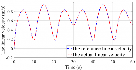
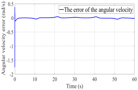
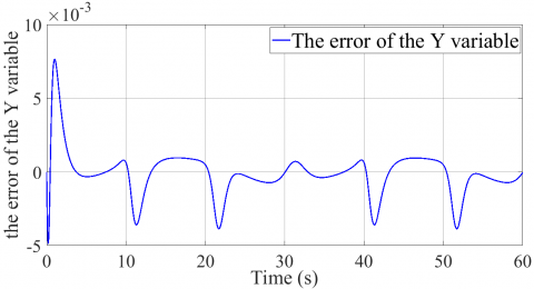
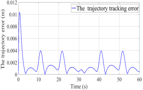
Figures 11(a)-11(c) display the desired and actual tracks for x, y, and $\theta$, respectively. The reference and actual amounts of the linear and angular speeds (v and w) are presented in Figures 12(a) and 12(b). However, Figures 13(a)-13(f) reveal the errors of the v, w, x, y, θ, and the tracking trajectory, respectively.
The HWGO-FOPID controller was designed to handle with the dynamics, which means a kinematic controller is necessary, therefore a back-stepping controller was proposed to guarantee a minimum of distance error that already has been proved in Figure 13(f) (error less than 0.004 m), this result demonstrate the reason behind the supposition of actual with the reference trajectories in Figures 10-12.
Figure 10. Star trajectory
(a)
(b)
(c)
Figure 11. Response of the (a) X; (b) Y; (c) θ variable
The addition of this controller in the external loop had influenced by decreasing the error of linear and angler velocity (the ISE of the HWGO) of the dynamic controller from 0.0452 to less than 0.002 as shown in Figures 13(a) and 13(b).
(a)
(b)
Figure 12. Response of (a) linear; and (b) angular Velocities (for star shape)
(a)
(b)
(c)
(d)
(e)
(f)
Figure 13. Error corresponding to (a) linear and (b) angular velocities; (c) x, (d) y and (e) theta variables; (f) the trajectory tracking
This paper presents an advanced optimization method to obtain the turning parameters of fractional order proportional integral derivative controller (FOPID controller). A comparison study was performed for the first time in the robotics field, where several tuning methods have been employed to set the details of two FOPID controllers, which are designed to make sure that the linear and angular speeds of the WMR follow the input reference. Those five meta-heuristics approached namely particle swarm optimizer (PSO), grey wolf optimizer (GWO), hybrid particle swarm grey wolf optimizer (HPSOGWO), whale optimizer (WOA) and hybrid grey wolf whale optimizer (HWGO) were found to be all statistically and graphically approved, by considering integral square error ISE as a cost function. A back-stepping kinematic controller was adopted to guarantee that tracking errors convergence to zero to achieve the trajectory tracking. A transient response in the time domain has been made to examine the performance of selected algorithms. Simulation results have successfully confirmed the over performance of HWGO in comparison to PSO, GWO, HPSOGWO, and WOA in terms of lowest error value obtained, convergence rapidity, with the minimum overshoot, received rise time, peak, peak time, and settling. Finally, a star trajectory demonstrated the robustness of the mentioned controller.
Chutarat Tearnbucha would like to acknowledge financial support by Navamindradhiraj University through the Navamindradhiraj University Research Fund (NURF).
[1] Zhang, L., Liu, L., Zhang, S. (2020). Design, implementation, and validation of robust fractional-order PD controller for wheeled mobile robot trajectory tracking. Complexity, 2020. https://doi.org/10.1155/2020/9523549
[2] Fue, K.G., Porter, W.M., Barnes, E.M., Rains, G.C. (2020). An extensive review of mobile agricultural robotics for field operations: Focus on cotton harvesting. AgriEngineering, 2(1): 150-174. https://doi.org/10.3390/agriengineering2010010
[3] Kot, T., Novák, P. (2018). Application of virtual reality in teleoperation of the military mobile robotic system TAROS. International Journal of Advanced Robotic Systems, 15(1): 1729881417751545. https://doi.org/10.1177%2F1729881417751545
[4] Arrshith, R.G., Suhas, K.S., Tejas, C., Subramaniyam, G. (2018). Unmanned ground vehicle (UGV)—Defense bot. In 2018 2nd International Conference on Inventive Systems and Control (ICISC), pp. 1201-1205. https://doi.org/10.1109/ICISC.2018.8398995
[5] Mihankhah, E., Kalantari, A., Aboosaeedan, E., Taghirad, H.D., Ali, S., Moosavian, A. (2009). Autonomous staircase detection and stair climbing for a tracked mobile robot using fuzzy controller. In 2008 IEEE International Conference on Robotics and Biomimetics, pp. 1980-1985. https://doi.org/10.1109/ROBIO.2009.4913304
[6] Hu, Y., Liu, R., Li, J., Yue, Y., Cheng, W., Zhang, P. (2014). Attenuation of collagen-induced arthritis in rat by nicotinic alpha7 receptor partial agonist GTS-21. BioMed Research International, 2014. https://doi.org/10.1155/2014/404059
[7] Murtaza, Z., Mehmood, N., Jamil, M., Ayaz, Y. (2014). Design and implementation of low cost remote-operated unmanned ground vehicle (UGV). In 2014 International Conference on Robotics and Emerging Allied Technologies in Engineering (iCREATE), pp. 37-41. https://doi.org/10.1109/iCREATE.2014.6828335
[8] Moon, H., Lee, J., Kim, J., Lee, D. (2009). Development of unmanned ground vehicles available of urban drive. In 2009 IEEE/ASME International Conference on Advanced Intelligent Mechatronics, pp. 786-790. https://doi.org/10.1109/AIM.2009.5229916
[9] Kaur, T., Kumar, D. (2015). Wireless multifunctional robot for military applications. In 2015 2nd International Conference on Recent Advances in Engineering & Computational Sciences (RAECS), pp. 1-5. https://doi.org/10.1109/RAECS.2015.7453343
[10] Al-Mayyahi, A., Wang, W., Birch, P. (2016). Design of fractional-order controller for trajectory tracking control of a non-holonomic autonomous ground vehicle. Journal of Control, Automation and Electrical Systems, 27(1): 29-42. https://doi.org/10.1007/s40313-015-0214-2
[11] Petre, E. (2002). An adaptive tracking controller for a mobile robot using neural networks. Journal of Control Engineering and Applied Informatics, 4(3): 25-32. https://doi.org/10.1016/j.neucom.2011.06.035
[12] Khai, T.Q., Ryoo, Y.J., Gill, W.R., Im, D.Y. (2020). Design of kinematic controller based on parameter tuning by fuzzy inference system for trajectory tracking of differential-drive mobile robot. International Journal of Fuzzy Systems, 22(6): 1972-1978. https://doi.org/10.1007/s40815-020-00842-9
[13] Khai, T.Q., Ryoo, Y.J. (2019). Design of adaptive kinematic controller using radial basis function neural network for trajectory tracking control of differential-drive mobile robot. International Journal of Fuzzy Logic and Intelligent Systems, 19(4): 349-359. https://doi.org/10.5391/IJFIS.2019.19.4.349
[14] Gheisarnejad, M., Khooban, M.H. (2019). Supervised control strategy in trajectory tracking for a wheeled mobile robot. IET Collaborative Intelligent Manufacturing, 1(1): 3-9.
[15] Esmaeili, N., Alfi, A., Khosravi, H. (2017). Balancing and trajectory tracking of two-wheeled mobile robot using backstepping sliding mode control: Design and experiments. Journal of Intelligent & Robotic Systems, 87(3): 601-613. https://doi.org/10.1007/s10846-017-0486-9
[16] Nikranjbar, A., Haidari, M., Atai, A.A. (2018). Adaptive sliding mode tracking control of mobile robot in dynamic environment using artificial potential fields. Journal of Computer & Robotics, 11(1): 1-14.
[17] Shanmugavel, M., Tsourdos, A., White, B., Żbikowski, R. (2010). Co-operative path planning of multiple UAVs using Dubins paths with clothoid arcs. Control Engineering Practice, 18(9): 1084-1092. https://doi.org/10.1016/j.conengprac.2009.02.010
[18] Fierro, R., Lewis, F.L. (1998). Control of a nonholonomic mobile robot using neural networks. IEEE Transactions on Neural Networks, 9(4): 589-600. https://doi.org/10.1109/72.701173
[19] Wang, G., Liu, X., Zhao, Y., Han, S. (2019). Neural network-based adaptive motion control for a mobile robot with unknown longitudinal slipping. Chinese Journal of Mechanical Engineering, 32(1): 1-9. https://doi.org/10.1186/s10033-019-0373-3
[20] Das, T., Kar, I.N. (2006). Design and implementation of an adaptive fuzzy logic-based controller for wheeled mobile robots. IEEE Transactions on Control Systems Technology, 14(3): 501-510. https://doi.org/10.1109/TCST.2006.872536
[21] Kumar, P., Chatterjee, S., Shah, D., Saha, U.K., Chatterjee, S. (2017). On comparison of tuning method of FOPID controller for controlling field controlled DC servo motor. Cogent Engineering, 4(1): 1357875. https://doi.org/10.1080/23311916.2017.1357875
[22] Bingul, Z., Karahan, O. (2018). Comparison of PID and FOPID controllers tuned by PSO and ABC algorithms for unstable and integrating systems with time delay. Optimal Control Applications and Methods, 39(4): 1431-1450. https://doi.org/10.1002/oca.2419
[23] Orman, K., Basci, A., Derdiyok, A. (2016). Speed and direction angle control of four wheel drive skid-steered mobile robot by using fractional order PI controller. Elektronika ir Elektrotechnika, 22(5): 14-19. https://doi.org/10.5755/j01.eie.22.5.16337
[24] Mishra, S.K., Chandra, D. (2014). Stabilization and tracking control of inverted pendulum using fractional order PID controllers. Journal of Engineering, 2014. https://doi.org/10.1155/2014/752918
[25] Bernardes, N.D., Castro, F.A., Cuadros, M.A., Salarolli, P.F., Almeida, G.M., Munaro, C.J. (2019). Fuzzy logic in auto-tuning of fractional PID and backstepping tracking control of a differential mobile robot. Journal of Intelligent & Fuzzy Systems, 37(4): 4951-4964. https://doi.org/10.3233/JIFS-181431
[26] Cajo, R., Mac, T.T., Plaza, D., Copot, C., De Keyser, R., Ionescu, C. (2019). A survey on fractional order control techniques for unmanned aerial and ground vehicles. IEEE Access, 7: 66864-66878. https://doi.org/10.1109/ACCESS.2019.2918578
[27] Aldair, A.A., Wang, W.J. (2010). Design of fractional order controller based on evolutionary algorithm for a full vehicle nonlinear active suspension systems. International Journal of Control and Automation, 3(4): 33-46.
[28] Rajesh, R. (2019). Optimal tuning of FOPID controller based on PSO algorithm with reference model for a single conical tank system. SN Applied Sciences, 1(7): 1-14. https://doi.org/10.1007/s42452-019-0754-3
[29] Ramezanian, H., Balochian, S., Zare, A. (2013). Design of optimal fractional-order PID controllers using particle swarm optimization algorithm for automatic voltage regulator (AVR) system. Journal of Control, Automation and Electrical Systems, 24(5): 601-611. https://doi.org/10.1007/s40313-013-0057-7
[30] Bhookya, J., Jatoth, R.K. (2019). Optimal FOPID/PID controller parameters tuning for the AVR system based on sine–cosine-algorithm. Evolutionary Intelligence, 12(4): 725-733. https://doi.org/10.1007/s12065-019-00290-x
[31] Verma, S.K., Yadav, S., Nagar, S.K. (2017). Optimization of fractional order PID controller using grey wolf optimizer. Journal of Control, Automation and Electrical Systems, 28(3): 314-322. https://doi.org/10.1007/s40313-017-0305-3
[32] Karam, Z.A., Awad, O.A. (2020). Design of active fractional PID controller based on whale's optimization algorithm for stabilizing a quarter vehicle suspension system. Periodica Polytechnica Electrical Engineering and Computer Science, 64(3): 247-263.
[33] Şenel, F.A., Gökçe, F., Yüksel, A.S., Yiğit, T. (2019). A novel hybrid PSO–GWO algorithm for optimization problems. Engineering with Computers, 35(4): 1359-1373. https://doi.org/10.1007/s00366-018-0668-5
[34] Singh, N., Singh, S.B. (2017). Hybrid algorithm of particle swarm optimization and grey wolf optimizer for improving convergence performance. Journal of Applied Mathematics, 2017. https://doi.org/10.1155/2017/2030489
[35] Korashy, A., Kamel, S., Jurado, F., Youssef, A.R. (2019). Hybrid whale optimization algorithm and grey wolf optimizer algorithm for optimal coordination of direction overcurrent relays. Electric Power Components and Systems, 47(6-7): 644-658. https://doi.org/10.1080/15325008.2019.1602687
[36] Fukao, T., Nakagawa, H., Adachi, N. (2000). Adaptive tracking control of a nonholonomic mobile robot. IEEE Transactions on Robotics and Automation, 16(5): 609-615. https://doi.org/10.1109/70.880812
[37] Fierro, R., Lewis, F.L. (1997). Control of a nonholomic mobile robot: Backstepping kinematics into dynamics. Journal of Robotic Systems, 14(3): 149-163.
[38] Ben Jabeur, C., Seddik, H. (2021). Design of a PID optimized neural networks and PD fuzzy logic controllers for a two‐wheeled mobile robot. Asian Journal of Control, 23(1): 23-41. https://doi.org/10.1002/asjc.2356
[39] Igor, P. (1999). Fractional-order systems and PIλDμ-controllers. IEEE Trans Autom Control, 44(1): 208-214. https://doi.org/10.1109/9.739144
[40] Bhookya, J., Jatoth, R.K. (2020). Fractional order PID controller design for multivariable systems using TLBO. Chemical Product and Process Modeling, 15(2). https://doi.org/10.1515/cppm-2019-0061
[41] Kennedy, J., Eberhart, R. (1948). Particle swarm optimization. In 1995 IEEE International Conference on Neural Networks Proceedings, 1: 6. https://doi.org/10.1109/ICNN.1995.488968
[42] Zorarpacı, E., Özel, S.A. (2016). A hybrid approach of differential evolution and artificial bee colony for feature selection. Expert Systems with Applications, 62: 91-103. https://doi.org/10.1016/j.advengsoft.2013.12.007
[43] Mittal, N., Singh, U., Sohi, B.S. (2016). Modified grey wolf optimizer for global engineering optimization. Applied Computational Intelligence and Soft Computing, 2016. https://doi.org/10.1155/2016/7950348
[44] Kishor, A., Singh, P.K. (2016). Empirical study of grey wolf optimizer. In Proceedings of Fifth International Conference on Soft Computing for Problem Solving, Springer, Singapore, pp. 1037-1049. https://doi.org/10.1007/978-981-10-0448-3_87
[45] Kirkpatrick, S., Gelatt, C.D., Vecchi, M.P. (1983). Optimization by simulated annealing. Science, 220(4598): 671-680.
[46] Osroush, M., Hosseini, S.A., Kamanbedast, A.A., Khosrojerdi, A. (2019). The effects of height and vertical position of slot on the reduction of scour hole depth around bridge abutments. Ain Shams Engineering Journal, 10(3): 651-659. https://doi.org/10.1016/j.asej.2019.10.003
[47] Kaur, G., Arora, S. (2018). Chaotic whale optimization algorithm. Journal of Computational Design and Engineering, 5(3): 275-284. https://doi.org/10.1016/j.jcde.2017.12.006
[48] Mohamed, M.J., Abbas, M.Y. (2018). Design a fuzzy PID controller for trajectory tracking of mobile robot. Engineering and Technology Journal, 36(1A). http://dx.doi.org/10.30684/etj.36.1A.15