Mustafa S. Abed* | Omar F. Lutfy | Qusay F. Al-Doori
© 2022 IIETA. This article is published by IIETA and is licensed under the CC BY 4.0 license (http://creativecommons.org/licenses/by/4.0/).
OPEN ACCESS
For autonomous mobile robots, determining the shortest path to the target is an indispensable requirement. In this work, two modifications of the Grey Wolf Optimization (GWO) method, which are called MGWO1 and MGWO2, are suggested for online path planning to make the mobile robot reach the goal using the shortest path and safely avoiding the obstacles in unknown environments. To avoid sharp curves, a cost function is derived using a path smoothing parameter and an integrated distance function. The results of the proposed approach are presented based on computer simulation in various unknown environments. A study was conducted to compare the performance of the proposed algorithm with those of other algorithms and the results indicated that the proposed GWO, MGWO1, and MGWO2 algorithms are competent in avoiding obstacles successfully including the local minima situation. Finally, the average enhancement rate in path length compared with Adaptive Particle Swarm Optimization (APSO), GWO is 5.30%, MGWO1 is 5.52%, and MGWO2 is 7.44%.
GWO, MGWO, path planning, mobile robot, obstacle avoidance
The motion planning issues of a mobile robot is an important topic of study in the area of mobile robots in current research [1]. Route planning is a process to obtain a sensible and collision-free route between the starting point and the destination, where the need to plan the route becomes important for a fully or partially automated process [2]. Generally, planning the movement of a mobile robot in an unfamiliar environment has been divided into two categories. First, the obstacles are unknown and the information about the obstacles is completely unknown. The most important thing in this situation is to avoid collisions with obstacles for mobile robots and not to seek the optimal planning of the movement. Second, the obstacles and their information are known [3]. Route planning can be divided into two categories: The first category is according to time, including online and offline planning. With online route planning, the route is calculated during movement based on sensor data, while with offline planning the route is calculated based on the environment model. The second category depends on the environment and it includes a dynamic environment that contains moving and static obstacles, while the static environment contains only static obstacles [4]. Many researchers have used different approaches in the navigation of Differential Wheel Mobile Robot (DWMR). For instance, Oleiwi et al. [5] applied fuzzy logic control for collision avoidance using only dynamic obstacles in partially unknown and known environments and they used the A-star algorithm to find the path in an offline manner. In another work [6], the authors proposed an intelligent Adaptive Particle Swarm Optimization (APSO) to be used for path planning in uncertain environments. Batti et al. [6] utilized fuzzy and neuro-fuzzy controllers to solve the simple static maze problem by obtaining information about some walls' positions in the maze using an offline approach. Gharajeh and Jond [7] employed an adaptive neuro-fuzzy network for a simple unknown static environment to find the best path. However, they did not apply their method in dynamic environments. Moreover, Pandey and Parhi [8] designed a fuzzy-wind-driven optimization algorithm that can deal with static and dynamic unknown environments. The drawback of this method cannot solve the local minima problem in U or L shape environment.
In general, while dealing with local route planning problems, the robot attempts to calculate its next collision-free point in an unknown area in steps from the start position to the finish position.
The robot position used in this study is based on the comparative location (Odometric Localization), where each robot calculates its following position based on its present position, angle, and speed over a certain period, as shown in Figure 1. In particular, the following position of the robot is calculated using Eqns. (1) and (2) [9].
$X_{\text {next }}=X_{\text {current }}+V \ln * \operatorname{Cos}\left(\theta_{i}\right)$ (1)
$Y_{\text {next }}=Y_{\text {current }}+V \ln * \sin \left(\theta_{i}\right)$, (2)
where, Xcurrent and Ycurrent are the coordinates of the current position and Xnext and Ynext are the coordinates of the succeeding nth robot position in the Cartesian coordinate. Moreover, the robot velocity, which is represented by vln and , θi represents the angle to direct the nth robot.
In this context, we need some criteria and rules to solve path-planning problems. These rules are explained below:
The start and goal positions of the mobile robot are predefined.
The robot uses its sensors to sense the nearby environment.
The path sensing and calculation from the start to the end position are accomplished in a counted number of steps by the robot.
The robot will directly navigate through its current and goal positions if the sensor detects no obstacles in the detection area, the robot goes to the goal position directly, otherwise, the proposed algorithm starts working to avoid obstacles, and then the robot goes to the goal position. Since the environment is unknown, the number of obstacles is unknown. Hence, the only limitation to the number of obstacles in the environment will be the processing ability of the simulation system.
All obstacles taken from the environment are circular, regardless of the shape of the obstacle and the area.
Figure 1. Next and current positions of the mobile robot
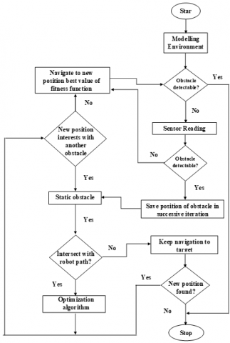
The route-planning model for the proposed system is shown in Figure 2.
Figure 2. Path planning model of the mobile robot
In this section, the Grey Wolf Optimization (GWO) method, and its two modified versions proposed in this work are explained in detail.
3.1 Grey Wolf Optimization (GWO)
The GWO algorithm is based on the natural leadership hierarchy and hunting mechanism of grey wolves. For simulating the leadership hierarchy, four types of grey wolves are used: alpha (α), beta $(\beta)$, delta ($\delta$), and omega (w). Furthermore, the three main steps of hunting are implemented including: searching for the prey, encircling the prey, and attacking the prey. There are mathematical models of the social hierarchy, as well as tracking, encircling, and attacking the prey [10].
3.1.1 The mathematical model in encircling the prey
Wolves encircle their victim when hunting. Eq. (3) and Eq. (4) are used to model this situation mathematically. The hunt with the new position of the grey wolves will be surrounded as a result of this:
$\vec{D}=|\vec{C} \cdot \overrightarrow{X p}(t)-\overrightarrow{X(t)}|$ (3)
$\vec{X}(l+1)=\overrightarrow{X p}(t)-\overrightarrow{A X} \cdot \overrightarrow{D X}$, (4)
where, $t$ indicates the present iteration $\overrightarrow{\boldsymbol{A}}$ and $\overrightarrow{\boldsymbol{C}}$ are coefficient vectors, $\overrightarrow{\boldsymbol{X} \boldsymbol{p}}$ is the prey position vector, and $\vec{X}$ indicates the grey wolf position vector. Eqs. $(5),(6)$, and (7) are used to $\vec{A}$, $\overrightarrow{\boldsymbol{C}}$ and $\overrightarrow{\boldsymbol{a}}$ :
$\vec{A}=2 \vec{a} \cdot \overrightarrow{r 1}-\vec{a}$ (5)
$\vec{C}=2 . \overrightarrow{r 1}$ (6)
$\vec{a}=2 *\left(1-\frac{l}{l_{\max }}\right)$, (7)
where, the components of $\vec{a}$ are linearly decreased from 2 to 0 over the course of iterations and $\overrightarrow{r 1}$ and $\overrightarrow{r 2}$ are random vectors in [0,1].
3.1.2 The mathematical model for hunting
Grey wolves have the ability to encircle victims. The mathematical model assumes that the prey does not know its location. As a result, alpha, beta, and delta have a better understanding of the prey's location. The three best candidate answers are alpha (the first best solution), followed by beta, and delta. Omega wolves reposition themselves in accordance with the upper layer wolves. In this approach, the following equations, namely Eq. (8), (9), and (10) are proposed:
$\overrightarrow{D \alpha}=|\overrightarrow{C 1 X} \cdot \overrightarrow{X \alpha}-\vec{X}|, \overrightarrow{D \beta}=|\overrightarrow{C 2} \cdot \overrightarrow{X \beta}-\vec{X}|\overrightarrow{D \delta}=|\overrightarrow{C 3} \cdot \overrightarrow{X \delta}-\vec{X}|$ (8)
$\overrightarrow{X 1}=\overrightarrow{X \alpha}-\overrightarrow{A 1} \cdot \overrightarrow{D \alpha}, \overrightarrow{X 2}=\overrightarrow{X \beta}-\overrightarrow{A 2} \cdot \overrightarrow{D \beta}\overrightarrow{X 3}=\overrightarrow{X \delta}-\overrightarrow{A 3} \cdot \overrightarrow{D \delta}$ (9)
$\vec{X}(l+1)=\frac{\overrightarrow{X 1}+\overrightarrow{X 2}+\overrightarrow{X 3}}{3}$ (10)
3.2 The modified GWO algorithm
In this work, two modifications were proposed to enhance the searching performance of the original algorithm. The first modification was considered according to Mittal et al. [11]. In particular, it is worth noticing that the exploration phase of the original GWO algorithm is relatively complicated. Therefore, an effective balance among the exploitation and the exploration abilities in the original GWO cannot be achieved by the simple linear parameter $\vec{a}$. As a result, a nonlinear parameter was suggested utilizing an exponential decay term. It is worth mentioning that the addition of the exponential decay function did not significantly increase the complexity of computation. On the other hand, adding this function has positively affected the convergence speed compared to the original algorithm. In particular, the adaptive parameter $\vec{a}$ is adjusted as expressed below [12]:
$\vec{a}=2 *\left(1-\frac{l^{k}}{l_{\max }^{k}}\right)$ (11)
The second modification was according to the ref. [12], in which proposing a nonlinear parameter that utilizes the cosine function so that the adaptibility of the $\vec{a}$ parameter is adjusted by [13]:
$\vec{a}=1-\cos \left(\left(1-\frac{l}{l_{\max }}\right)^{k} * \pi\right)$ (12)
where, lmax denotes the maximum number of iterations and l is the current iteration. k=2 is the nonlinear adjustment parameter. For comparison purposes, the algorithms with the first and the second modifications were called MGWO1 and MGWO2, respectively.
Despite the modifications above, the optimal path increases in length in our application, and thus another modification on Eq. (10) was required. Particularly, the location vector of a grey wolf in the original GWO algorithm is equally guided by the positions of $\alpha, \beta$, and $\delta$ wolves as provided by Eq. (10). In this work, to calculate the location vector of a grey wolf, a more weight value is given to α wolf followed by the $\beta$ and the $\delta$ wolfs in the proposed modification, as follows:
$\vec{X}(l+1)=\frac{\overrightarrow{w 1 * X 1}\quad+\quad\overrightarrow{w 2 * X 2}\quad+\quad\overrightarrow{w 3 * X 3}}{6}$ (13)
where, $w 1, w 2$, and $w 3$ are the variable weight values for the $\alpha, \beta$, and $\delta$ wolves, respectively. First of all, the summation of the weights should equal $1.0[13]$, that is:
$\mathrm{w}_{1}+\mathrm{w}_{2}+\mathrm{w}_{3}=1$ (14)
Secondly, the weights of the alpha wolf w1, the beta wolf w2, and the delta wolf w3 should always satisfy $w 1 \geq w 2 \geq w 3$. Specifically, these weights were selected based on trial and error bases in this work to achieve the desired performance.
For safety purposes, the distance between the mobile robot and the obstacle must be kept to the maximum. On the other hand, the distance from the robot to the goal must be minimal to achieve the shortest path. Based on the two perspectives above, the cost function is designed to guarantee the optimal path. Particularly, the cost function has the following equation [14]:
Cost Function $=\left[\alpha_{1} \times d R G+\alpha_{2} \div d R O+\alpha_{3} \times \theta\right]$ (15)
where, the parameter α1 is set so that the robot covers the minimum distance and reaches the target point as soon as possible [14]. Similarly, α2 controls the distance between the robot and the obstacle. α3 represents the path smoothing term utilized in the cost function so that the robot can avoid sharp turns in the suggested technique.
dRO and dRG are used to calculate the distance between the robot and the obstacles and the distance between the robot and the destination point, respectively, and the Euclidean distance equation is employed as given below:
$d R O=\sqrt{(X o b s-X r)^{2}+(Y o b s-Y r)^{2}}$ (16)
$d R G=\sqrt{(X g-X r)^{2}+(Y g-Y r)^{2}}$ (17)
In addition, θ is the deviation angle desired by the robot to detect the next position in the environment. Specifically, θ is given by Eq. (17).
$\theta=\tan ^{-1} \frac{Y g-Y r}{X g-X r}$ (18)
where, Xg and Yg are the goal's coordinates in the x and y environment, Xr and Yr are the current robot's coordinate x and y values, and Xobs and Yobs are the obstacle's coordinates x and y in the environment.
The complete flowchart of the proposed algorithm is presented in Figure 3.
Figure 3. Flowchart of the optimization procedure
Using MATLAB R2016 b, the simulation tests were performed in a PC of Windows 10 OS, Intel(R) Core (TM) i7-8550 U processor, 1.80 GHz CPU, and 20 GB RAM. The simulation parameters considered for the proposed algorithm are listed in Table 1.
Table 1. Parameter settings for the simulation
|
Parameters used in optimization |
|
|
Number of search agents |
10 |
|
Maximum number of iterations |
10 |
|
Dimension |
1 |
|
Lower bound |
-5 |
|
Upper bound |
5 |
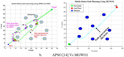
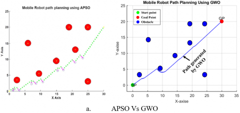
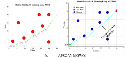
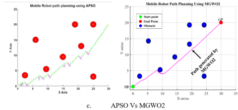
Figures 4, 5, 6, 7, and 8 show the best simulation results obtained by the proposed method when various situations are considered and compared to the APSO in reference [14]. Moreover, Figure 9 shows an environment that contains more than 30 unknown obstacles and this environment has been built in this work to demonstrate the effectiveness of the proposed approach. In this environment, the two modified versions, namely MWOG1 and MWOG2, were compared with the original GWO. To take into account the random nature of the above algorithms, 10 runs were performed for each algorithm and the average performance was considered.
Table 2 shows the average path distance including the path lengths and time duration for the robot while utilizing the suggested method and the APSO. The suggested method clearly outperforms the APSO based on the tabulated data.
Table 3 illustrates the enhancement rates in the path length for the modified algorithms compared to the APSO. In addition, the enhancement rates in the path length compared to the original GWO are shown in Table 4.
Figure 10 depicts the path lengths generated by each algorithm for all maps, while Figure 11, depicts the execution times taken by each algorithm for all maps.
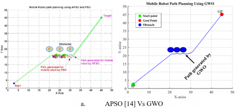
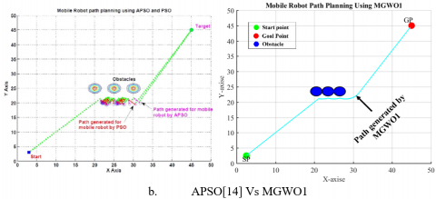
Figure 4. Simulation graph for single obstacle environment with a starting point at (2.5,2.5) and an endpoint at (45,45) :(a) APSO[14] Vs AGWO (b) APSO[14] Vs MGWO1 (c) APSO[14] MGWO2
Figure 5. Simulation graph in obstacle avoidance in a narrow escaping environment with a starting point at (2.5,2.5) and an endpoint at (45,45): (a) APSO[14] Vs AGWO ( b) APSO[14] Vs MGWO1 (c) APSO[14] MGWO2
Figure 6. Simulation graph obstacle avoidance in trap condition with a starting point at (2.5,2.5) and ab endpoint at (45,45): (a) APSO[14] Vs AGWO (b) APSO[14] Vs MGWO1 (c) APSO[14] MGWO2
Figure 7. Simulation graph of local minima environment with a starting point at (2.5,2.5) and an endpoint at (45,45): (a) APSO[14] Vs AGWO ( b) APSO[14] Vs MGWO1 (c) APSO[14] MGWO2
Figure 8. Simulation graph obstacle avoidance in a maze environment with a starting point at (0,0) and an endpoint at (30,20): (a) APSO[14] Vs AGWO ( b) APSO[14] Vs MGWO1 (c) APSO[14] MGWO2
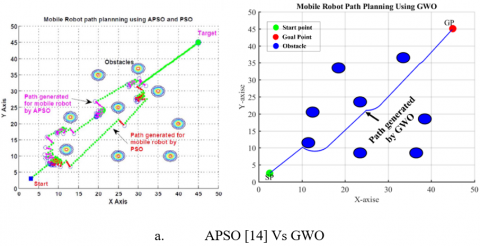
Figure 9. Simulation graph of the complex environment have obstacle more than 30 with a starting point at (2.5,2.5) and an endpoint at (45,45) GWO vs MGWO 1 Vs MGWO2
Table 2. Results of the average path lengths and average execution times
|
Figure Number |
Map |
Average Path length in pixels |
Average Time in sec |
||||||
|
[14] |
GWO |
MGWO1 |
MGWO2 |
[14] |
GWO |
MGWO1 |
MGWO2 |
||
|
4 |
Map (1) |
1288.25 |
1211.04497 |
1206.62925 |
1204.15383 |
43.85 |
47.85829 |
50.20214 |
48.04653 |
|
5 |
Map (2) |
1285.56 |
1249.10671 |
1245.55649 |
1240.21618 |
68.05 |
76.45092 |
75.34207 |
82.26741 |
|
6 |
Map (3) |
2237.31 |
2223.36704 |
2218.05451 |
2215.48116 |
57.87 |
68.56733 |
72.63015 |
67.80567 |
|
7 |
Map (4) |
1784.71 |
1692.208 |
1687.231 |
1529.83347 |
64.87 |
110.4472 |
107.06874 |
108.12077 |
|
8 |
Map (5) |
470.45 |
414.6995 |
414.75093 |
414.4694 |
XX |
34.47171 |
32.23354 |
36.02424 |
|
9 |
Map (6) |
XX |
439.19928 |
434.33948 |
433.9618 |
XX |
61.74871 |
89.49583 |
83.12656 |
Table 3. Enhancement rates in the path lengths compared to the APSO
|
Figure Number |
Map |
Enhancement rate in path length |
||
|
GWO |
MGWO1 |
MGWO2 |
||
|
4 |
Map (1) |
5.99302% |
6.33578% |
6.52794% |
|
5 |
Map (2) |
2.8356% |
3.11176% |
3.52716% |
|
6 |
Map (3) |
0.6232% |
0.860654% |
0.975673% |
|
7 |
Map (4) |
5.18303% |
5.4619% |
14.2811% |
|
8 |
Map (5) |
11.8505% |
11.8395% |
11.8994% |
Table 4. Enhancement rates in the path lengths compared to the original GWO
|
Figure Number |
Map |
Enhancement rate of path length |
|
|
MGWO1 |
MGWO2 |
||
|
4 |
Map (1) |
0.364621% |
0.569024% |
|
5 |
Map (2) |
0.284221% |
0.711751% |
|
6 |
Map (3) |
0.238941% |
0.354682% |
|
7 |
Map (4) |
0.294113% |
9.59542% |
|
8 |
Map (5) |
0.0124018% |
0.055486% |
|
9 |
Map (6) |
1.10651% |
1.19251% |
Figure 10. Path lengths are generated by each algorithm for all maps
Figure 11. Execution times were taken by each algorithm for all maps
To demonstrate the ability of the proposed algorithm to handle unknown environments, obstacles were implanted in the optimal path of the mobile robot. Figures (4,5,6,7,8, and 9) show that the mobile robot recognizes the obstacle and measures its dimensions then predicts the new path which avoids the implanted obstacles.
The proposed algorithms have been successfully implemented for online mobile robot navigation in simulated environments. Specifically, the original GWO algorithm and two other modified versions, namely MGWO1 and MGWO2, were exploited to find the shortest path in unknown environments. we apply all algorithms in a different case with complex in obstacle more than 30 obstacles the algorithms work successfully. In particular, the original GWO algorithm-generated shorter paths with less time compared to the APSO as shown the average enhancement rate in path length compared with (APSO) is 5.30%. Moreover, the MGWO1 and MGWO2 resulted in shorter paths and less execution time compared to the APSO. The average enhancement rate was 5.52%, and 7.44% of MGWO1 and MGWO2 respectively with APSO.The 0.38%, 2.08% of MGWO1 and MGWO2 respectively with the original GWO.As for the modified versions, the MGWO2 generated shorter paths with shorter execution times compared to the MGWO1 due to the presence of the cosine function in the MGWO2. It is worth mentioning that the proposed algorithms can be utilized for environments with dynamic obstacles and several mobile robots.
[1] Oleiwi, B.K., Roth, H., Kazem, B.I. (2014). A hybrid approach based on ACO and GA for multi objective mobile robot path planning. In Applied Mechanics and Materials, 527: 203-212. https://doi.org/10.4028/www.scientific.net/AMM.527.203
[2] Raheem, F.A., Hameed, U.I. (2018). Interactive heuristic D* path planning solution based on pso for two-link robotic arm in dynamic environment. World Journal of Engineering and Technology, 7(1): 80-99. https://doi.org/10.4236/wjet.2019.71005
[3] Oleiwi, B.K., Al-Jarrah, R., Roth, H., Kazem, B.I. (2014). Multi objective optimization of trajectory planning of non-holonomic mobile robot in dynamic environment using enhanced GA by fuzzy motion control and A. In International Conference on Neural Networks and Artificial Intelligence, pp. 34-49. https://doi.org/10.1007/978-3-319-08201-1_5
[4] Shwail, S.H., Karim, A. (2014). Probabilistic roadmap, A*, and GA for proposed decoupled multi-robot path planning. Iraqi Journal of Applied Physics, 10(2): 3-9.
[5] Oleiwi, B.K., Mahfuz, A., Roth, H. (2021). Application of fuzzy logic for collision avoidance of mobile robots in dynamic-indoor environments. In 2021 2nd International Conference on Robotics, Electrical and Signal Processing Techniques (ICREST), pp. 131-136. https://doi.org/10.1109/ICREST51555.2021.9331072
[6] Batti, H., Ben Jabeur, C., Seddik, H. (2021). Autonomous smart robot for path predicting and finding in maze based on fuzzy and neuro‐fuzzy approaches. Asian Journal of Control, 23(1): 3-12. https://doi.org/10.1002/asjc.2345
[7] Gharajeh, M.S., Jond, H.B. (2020). Hybrid global positioning system-adaptive neuro-fuzzy inference system based autonomous mobile robot navigation. Robotics and Autonomous Systems, 134: 103669. https://doi.org/10.1016/j.robot.2020.103669
[8] Pandey, A., Parhi, D.R. (2017). Optimum path planning of mobile robot in unknown static and dynamic environments using fuzzy-wind driven optimization algorithm. Defence Technology, 13(1): 47-58. https://doi.org/10.1016/j.dt.2017.01.001
[9] Malu, S.K., Majumdar, J. (2014). Kinematics, localization and control of differential drive mobile robot. Global Journal of Research In Engineering, 14(1).
[10] Mirjalili, S., Mirjalili, S.M., Lewis, A. (2014). Grey wolf optimizer. Advances in Engineering Software, 69: 46-61. https://doi.org/10.1016/j.advengsoft.2013.12.007
[11] Mittal, N., Singh, U., Sohi, B.S. (2016). Modified grey wolf optimizer for global engineering optimization. Applied Computational Intelligence and Soft Computing, 2016.
[12] Gai, W., Qu, C., Liu, J., Zhang, J. (2018). An improved grey wolf algorithm for global optimization. In 2018 Chinese Control And Decision Conference (CCDC), 2494-2498.
[13] Gao, Z.M., Zhao, J. (2019). An improved grey wolf optimization algorithm with variable weights. Computational Intelligence and Neuroscience, 2019. https://doi.org/10.1155/2019/2981282
[14] Mohanty, P.K., Dewang, H.S. (2021). A smart path planner for wheeled mobile robots using adaptive particle swarm optimization. Journal of the Brazilian Society of Mechanical Sciences and Engineering, 43(2): 1-18. https://doi.org/10.1007/s40430-021-02827-7