Nadia Bounouara | Mouna Ghanai | Kheireddine Chafaa*
© 2021 IIETA. This article is published by IIETA and is licensed under the CC BY 4.0 license (http://creativecommons.org/licenses/by/4.0/).
OPEN ACCESS
In this paper, the Particle Swarm Optimization algorithm (PSO) is combined with Proportional-Derivative (PD) and Proportional-Integral-Derivative (PID) to design more efficient PD and PID controllers for robotic manipulators. PSO is used to optimize the controller parameters Kp (proportional gain), Ki (integral gain) and Kd (derivative gain) to achieve better performances. The proposed algorithm is performed in two steps: (1) First, PD and PID parameters are offline optimized by the PSO algorithm. (2) Second, the obtained optimal parameters are fed in the online control loop. Stability of the proposed scheme is established using Lyapunov stability theorem, where we guarantee the global stability of the resulting closed-loop system, in the sense that all signals involved are uniformly bounded. Computer simulations of a two-link robotic manipulator have been performed to study the efficiency of the proposed method. Simulations and comparisons with genetic algorithms show that the results are very encouraging and achieve good performances.
Particle Swarm Optimization (PSO), PD controller, PID controller, robotic manipulators
In the literature we can find different types of controllers like PD; PI and PID where they are designed to stabilize dynamical systems. PD is one of the most important controllers and it is extensively used in different industry areas. PID is a combination of proportional, derivative and integral actions. It is an important element for distributed process control systems. Modern PID controllers are endowed with adaptive systems which can tune their free parameters. Note that PID controller acts in a very smooth and progressive manner, making sharp changes to consider the small deviations to correct rapid perturbations. Note also that PD and PID controllers are able to achieve the position control objective for robotic systems by calculating the error between the measured and the desired variables and minimizing the error by adjusting their parameters [1].
Optimization is a very important tool in engineering; it is the act of obtaining the best result under given circumstances such as design, construction or maintenance. The main objective of all such tools is the extremization, which is the process of finding the minimum or maximum value of a function.
In controller design, parameters tuning is crucial, which gives the best performances for the system. There are various parameter optimization methods, and it is generally very difficult to choose the best ones due to the performance of each method being a problem-dependent [2, 3].
Among the important optimization methods used in parameters optimization we find: least squares method [4], gradient descent [5], Genetic Algorithm (GA) [6-9], Particle Swarm Optimization (PSO) [8, 10-13], Differential Evolution (DE) [7, 14-16], and Gray Wolf Optimization (GWO) [17]. Sharma et al. [9] have applied GA algorithm to a two-link planar rigid robotic manipulator for optimization of PID controller gains. Laamari et al. [12] have proposed an effective approach PSO-EKF to optimize the speed and rotor flux of an induction motor drive. Mohanty et al. [16] have applied DE technique to obtain the PID controller parameters. Tripathi et al. [17] have considered the optimization error to estimate the best appropriate PID parameters.
PSO algorithm is an innovative distributed intelligent paradigm for solving optimization problems that originally took its inspiration from biological examples by swarming, flocking and herding phenomena in vertebrates. PSO incorporates swarming behaviors observed in flocks of birds, schools of fish, or swarms of bees, and even human society, from which the idea is emerged [18, 19]. Recently, many modified and improved versions of PSO was proposed in the literature, such as Simplified Particle Swarm Optimization (SPSO) [20], Modified Particle Swarm Optimization (MPSO) [21] and Improved Particle Swarm Optimization (IPSO) [22, 23].
In this paper, we introduce a new alternative to tune PD and PID parameters based on PSO optimization algorithm by optimizing the objective function defined by Mean Absolute Error (MAE). Minimizing the MAE is usually considered as a good performance index designing, and its optimization will adjust PD and PID parameters ${{K}_{p}}$, ${{K}_{i}}$ and ${{K}_{d}}$. Note that optimization process is constrained in order to guarantee the stability of the system by using Lyapunov stability method. In this investigation we propose an alternative for the adaptation and optimization of ${{K}_{p}}$, ${{K}_{i}}$ and ${{K}_{d}}$. For this propose we suggest to combine PSO with PID and PD in order to improve their performance.
Inertia weight is a crucial parameter of the PSO algorithm which allows controlling its convergence. Two different inertia weights are considered in this paper: Constant Inertia Weight (CIW), and Variable Inertia Weight (VIW) which give us two strategies PSOCIW and PSOVIW. The aim of this investigation is to apply these two strategies for the optimization of PID (PD) free parameters to control a robotic system.
The framework of the proposed method is made of two steps. In the first step, which is an offline stage, PSO optimizer will find the optimal PD and PID parameters ${{K}_{p}}$, ${{K}_{i}}$ and ${{K}_{d}}$. In the second step, we take the estimated parameters obtained in step one and inject them into the control loop.
The rest of the paper is organized as follows: The design of PD and PID controllers is described in Section 2. Section 3 presents the principle concepts of PSO algorithm. Simulation example is given in Section 4. Finally, conclusions are given in Section 5.
PD and PID parameters are chosen according to the system to be considered. Thus, their optimal values are very necessary to guarantee the desired performance.
The nth degree robot manipulator dynamic is represented by the following differential equation [24].
$H(q)\ddot{q}+C(q,\dot{q})\dot{q}+g(q)=\tau $ (1)
where, $H(q)$ an $n\times n$ symmetric, positive definite mass matrix; $C(q,\dot{q})\dot{q}$ is the torques due to centrifugal forces; $g(q)$ is the gravity forces; $\tau $ is the $n\times 1$vector of joint torques supplied by the actuators; $q$ is the $n\times 1$ vector of joint displacements.
2.1 Design of PD controller
PD controller framework is shown in Figure 1, where its control action is defined to be:
$\begin{align} & \tau ={{K}_{p}}\left( {{q}_{d}}-q \right)+{{K}_{d}}\left( {{{\dot{q}}}_{d}}-\dot{q} \right)+g(q) \\ & \,\,\,\,={{K}_{p}}e+{{K}_{d}}\dot{e}+g(q) \\ \end{align}$ (2)
where, ${{q}_{d}}$ is the desired position vector; ${{\dot{q}}_{d}}$ the desired velocity vector; $e={{q}_{d}}-q$ the position error vector and $\dot{e}={{\dot{q}}_{d}}-\dot{q}$ is velocity error vector.
Note that ${{q}_{d}}$ and ${{\dot{q}}_{d}}$ are compared to the actual position $q$ and the actual velocity $\dot{q}$, respectively; and then the differences are multiplied by a position gain ${{K}_{p}}$ and a velocity gain ${{K}_{d}}$ to generate the control torque (2).
Figure 1. Structure of PD controller
Note that an asymptotic tracking of the desired position is assured by law (2). Let the following Lyapunov function candidate:
$\nu =\frac{1}{2}{{\dot{q}}^{T}}H(q)\dot{q}+\frac{1}{2}{{e}^{T}}{{K}_{p}}e$ (3)
Lyapunov function (3) represents the total energy of the manipulator and it is always positive or equal to zero due to the positiveness of matrices $H(q)$ and ${{K}_{p}}$. The time derivative of $v$ is:
$\dot{\nu }={{\dot{q}}^{T}}H(q)\ddot{q}+\frac{1}{2}{{\dot{q}}^{T}}\dot{H}(q)\dot{q}-{{\dot{q}}^{T}}{{K}_{p}}e$ (4)
Combining (1) and (4) gives:
$\begin{align} & \dot{\nu }={{{\dot{q}}}^{T}}\left( \tau -C\left( q,\dot{q} \right)\dot{q}-g(q) \right)+\frac{1}{2}{{{\dot{q}}}^{T}}\dot{H}(q)\dot{q}-{{{\dot{q}}}^{T}}{{K}_{p}}e \\ & \,\,\,\,={{{\dot{q}}}^{T}}\left( \tau -g(q)-{{K}_{p}}e \right)+\frac{1}{2}{{{\dot{q}}}^{T}}\left( \dot{H}(q)-2C\left( q,\dot{q} \right) \right)\dot{q} \\ & \,\,\,\,={{{\dot{q}}}^{T}}\left( \tau -g(q)-{{K}_{p}}e \right) \\ \end{align}$ (5)
where we have used the fact that $\dot{H}-2C$ is skew symmetric. Substituting PD control law (2) into (5) gives:
$\dot{\nu }=-{{\dot{q}}^{T}}{{K}_{d}}\dot{q}\le 0$ (6)
The above analysis show that $v$ decreases as long $\dot{q}$ is nonzero. In the case of $\dot{\nu }=0$, (6) then implies that $\dot{q}\equiv 0$ and hence $\ddot{q}\equiv 0$. Using the dynamical Eq. (1) and the PD control (2) we obtain:
$H(q)\ddot{q}+C(q,\dot{q})\dot{q}+g(q)={{K}_{p}}e-{{K}_{d}}\dot{q}+g(q)$ (7)
then ${{K}_{p}}e\equiv 0$ and because ${{K}_{p}}$ is nonsingular, we have $e\equiv 0$.
Therefore, control low (2) applied to the system (1) achieves global asymptotic stability and the robot is therefore well-stabilized by the addition of PD-type control law.
2.2 Design of PID controller
A PID torque control for the robot manipulator (1) is shown in Figure 2 and given by
$\begin{align} & \tau ={{K}_{p}}\left( {{q}_{d}}-q \right)+{{K}_{i}}\int{\left( {{q}_{d}}-q \right)}\,dt \\ & \,\,\,\,\,\,\,+{{K}_{d}}\left( {{{\dot{q}}}_{d}}-\dot{q} \right)+g(q) \\ & \,\,\,\,={{K}_{p}}e+{{K}_{i}}\int{e}\,dt-{{K}_{d}}\dot{q}+g(q) \\ \end{align}$ (8)
where, ${{K}_{p}}$, ${{K}_{i}}$ and ${{K}_{d}}$ are the PID parameters to be tuned to achieve an accepted level of performance.
The kinetic energy of the manipulator is the scalar function which is represented in terms of the generalized coordinates and their derivatives as
$K=\frac{1}{2}{{\dot{q}}^{T}}H(q)\dot{q}$ (9)
Figure 2. Structure of PID controller
The potential energy is expressed in terms of the generalized coordinates using the relationship.
$P={{q}^{T}}{{r}_{c}}m$ (10)
where, ${{r}_{c}}\in {{\Re }^{n}}$; $m$ denotes the mass.
Defining $\dot{q}=\omega $ where $\omega \in {{\Re }^{n}}$ denotes the angular velocity vector.
Let rewrite (1) as:
$\dot{\omega }=-H{{(q)}^{-1}}\left[ C(q,\omega )\omega +g(q)-\tau \right]$ (11)
The PID control function (8) becomes:
$\tau ={{K}_{p}}({{q}_{q}}-q)+{{K}_{i}}\int{({{q}_{q}}-q)}\,dt-{{K}_{d}}\omega +g(q)$ (12)
Eq. (2) imply that the resulting system is expressed as:
$\begin{align} & \dot{\omega }=-H{{(q)}^{-1}}(C(q,\omega )\omega -{{K}_{p}}({{q}_{q}}-q) \\ & \,\,\,\,\,\,\,\,\,-{{K}_{i}}\int{({{q}_{q}}-q)}\,dt+{{K}_{d}}\omega +g(q)) \\ \end{align}$ (13)
Let the following Lyapunov function candidate,
$\begin{align} & \nu \left( q,\omega \right)=\frac{1}{2}{{q}^{T}}{{K}_{q}}q+{{q}^{T}}{{K}_{q\omega }}\omega \\ & \,\,\,\,\,\,\,\,\,\,\,\,\,\,\,\,\,\,\,\,+\frac{1}{2}{{\omega }^{T}}H(q)\omega +{{q}^{T}}{{r}_{c}}m \\ \end{align}$ (14)
where, ${{K}_{q}}\in {{\Re }^{n\times n}}$ and ${{K}_{q\omega }}\in {{\Re }^{n\times n}}$ are positive-definite matrices.
The time derivative of $v$ is:
$\begin{align} & \dot{\nu }\left( q,\omega \right)={{{\dot{q}}}^{T}}{{K}_{q}}q+\dot{q}{{K}_{q\omega }}\omega +{{q}^{T}}{{K}_{q\omega }}\dot{\omega } \\ & \,\,\,\,\,\,\,\,\,\,\,\,\,\,\,\,\,\,\,+{{{\dot{\omega }}}^{T}}H(q)\omega +\frac{1}{2}{{\omega }^{T}}\dot{H}(q)\omega +{{r}_{c}}m \\ \end{align}$ (15)
According to Eq. (13) and Eq. (15) and because $H(q)$ is positive definite matrix, therefore it follows at once that $\dot{\nu }\left( q,\omega \right)$ is negative definite.
Particle Swarm Optimization (PSO) is an evolutionary computation technique inspired by social behavior of groups like bird flocking, fish schooling or colonies of insects; because it is known that a group can effectively achieve an objective by using the common information of every element. PSO algorithm was first introduced in 1995 by Eberhart and Kennedy [25] as an alternative to population based search approaches (like genetic algorithms) in order to solve optimization problems.
In this algorithm the elements of the population are called particles, and each particle (a bird or a fish) is a candidate for the solution. Each particle is considered as a moving point in the N-dimensional search space with a certain velocity. The velocity of each particle is constantly adjusted according to its own experience and the experience of its companions hopping to fly towards better solution area.
In PSO, each state of particle presents a position and velocity, which is initialized with a population generation by a random process. Note that each particle is described by three features:
$x_{k}^{i}$: ${{i}^{th}}$ particle vector position at time $k$.
$v_{k}^{i}$: ${{i}^{th}}$ particle velocity at time $k$, which represents the search direction and used to update the position vector.
$J\left( x_{k}^{i} \right)$: fitness or objective, determines the best position of each particle over time.
Mathematically, the particle velocities are updates according to the following equations:
$v_{k+1}^{i}=wv_{k}^{i}+{{c}_{1}}rand({{p}^{i}}-x_{k}^{i})+{{c}_{2}}rand(p_{k}^{g}-x_{k}^{i})$ (16)
where, $v_{k+1}^{i}$ is the new velocity, $w$ the inertia factor, ${{c}_{1}}$ positive constant (self confidence), ${{c}_{2}}$ positive constant (swarm confidence), symbol $g$ represents the index of best particle among all the particles in the population, ${{p}^{i}}$ ${{i}^{th}}$ particle best position (the best position in the swarm), $p_{k}^{g}$ particle best global position (best particle among all the particles in the population) until time $k$(so, ${{p}^{g}}$ will be the last best global position), $rand$ is a random number uniformly distributed in $\left[ 0,\,\,1 \right]$.
Particle positions are the updates by velocity (16) as:
$x_{k+1}^{i}=x_{k}^{i}+v_{k+1}^{i}$ (17)
The PSO principle consists of, at each time step, regulating the velocity and location of each particle toward its ${{p}^{i}}$ and ${{p}^{g}}$ locations according to Eq. (16) and Eq. (17) until a maximum change in the fitness function will be smaller than a specified tolerance $\varepsilon $ which gives us the following stopping criteria.
$\left| J\left( p_{k+1}^{g} \right)-J\left( p_{k}^{g} \right) \right|\le \varepsilon $ (18)
The following algorithm provides a brief summary of the PSOVIW algorithm 1.
Algorithm 1
Begin Algorithm
Input: function to optimize, $J$
swarm size, $N$
problem dimension, $D$
Output: ${{x}^{*}}$ the best value found
Initialize: for all particles in problem space
${{x}_{i}}=\left( {{x}_{i1}},\ldots ,{{x}_{iD}} \right)$ and ${{v}_{i}}=\left( {{v}_{i1}},\ldots ,{{v}_{iD}} \right)$,
Evaluate $J\left( {{x}_{i}} \right)$in $D$variables and get$pbes{{t}_{i}}$, $\left( i=1,\ldots ,N \right)$
$gbest$ ← $pbes{{t}_{i}}$
Repeat
Calculate $VIW$using (20)
Update ${{v}_{i}}$ for all particles using (16)
Update ${{x}_{i}}$ for all particles using (17)
Evaluate $J\left( {{x}_{i}} \right)$ in $D$variables and get $pbes{{t}_{i}}$,
$\left( i=1,\ldots ,N \right)$
If $J\left( {{x}_{i}} \right)$ is better than $pbes{{t}_{i}}$ then $pbes{{t}_{i}}$ ← ${{x}_{i}}$
If the $pbes{{t}_{i}}$ is better than $gbest$ then $gbest$← $pbes{{t}_{i}}$
Until stopping criteria (e.g., maximum iteration or error tolerance is met)
${{x}^{*}}$← $gbest$
Return ${{x}^{*}}$
End Algorithm
The PID or PD problematic is that its control is greatly affected by the parameters${{K}_{p}}$, ${{K}_{i}}$ and ${{K}_{d}}$. Bad choice for these parameters will make the result of tracking divergent or will give large errors. To surmount this difficulty and to obtain the best performances, ${{K}_{p}}$, ${{K}_{i}}$ and ${{K}_{d}}$ have to be considered as free parameters to be adapted. The tuning of ${{K}_{p}}$, ${{K}_{i}}$ and${{K}_{d}}$ will affect both the transient time interval and steady-state operation of the response.
PID or PD parameters have to be optimized with a very high accuracy in order to obtain precise response. This task is very difficult due to the probable unknown system dynamics. To elucidate this problematic, controller parameter must be considered as free parameters to be adjusted. In the literature, the considered parameters were first tuned or adjusted by trial and error method which was a very hard task which takes longue time. In order to surmount this difficulty and to avoid trial and error method, PSO with Variable Inertia Weight $w$, in which it will be decreased linearly with the iteration number (PSOVIW) technique, was used to tune and optimize the controller parameters automatically.
In this section, we propose a new alternative for the adaptation and optimization of ${{K}_{p}}$, ${{K}_{i}}$ and ${{K}_{d}}$ based on the PSOVIW algorithm in order to eliminate the steady-state error, reduce the overshoot amplitude and decrease the rise time. For this purpose, we suggest to combine PSOVIW optimization with PID or PD in order to design an efficient PID (PD) for two link robot manipulators. To our knowledge, this work has not been done before. The framework of the proposed method is made of two steps. In the first step represented in Figure 3, we present a PSOVIW-PID (PD) combination working in an offline way to optimize the optimal values of ${{K}_{p}}$, ${{K}_{i}}$ and ${{K}_{d}}$. In the second step, we take the optimized quantities from step one and insert them into the online PID (PD) controller of two link robot manipulator parameters.
The structure of the PSOVIW-PID (PD) parameter optimization system is illustrated in Figure 3. We consider that the input of the system is the vector $r\left( t \right)={{\left[ \begin{matrix} {{\theta }_{d1}} & {{\theta }_{d2}} \\\end{matrix} \right]}^{T}}$ and the measured response is $y={{\left[ \begin{matrix} {{\theta }_{1}} & {{\theta }_{2}} \\\end{matrix} \right]}^{T}}$ obtained by an angle sensor (encoder). Note that the error between $r$ and $y$ is set to be an input for the PID (PD) as well as the optimized parameters ${{K}_{p}}$, ${{K}_{i}}$ and ${{K}_{d}}$. Actual tracking errors are used by the performance evaluator. The performance evaluator estimates the objective function which is a Mean Absolute Error (MAE) criterion between the actual output and the desired reference input defined in what follows:
$J=MAE=\frac{1}{N}\left( \sum\limits_{k=1}^{N}{\sum\limits_{i=1}^{2}{\left| {{e}_{i,k}} \right|}} \right)$ (19)
where, $i=1,\,2$ is the number of robot articulations and $N$ is the number of data samples, such that:
${{e}_{1}}=\left\{ {{\theta }_{1d}}(k)-{{\theta }_{1}}(k) \right\}$ is the output error of the first articulation;
${{e}_{2}}=\left\{ {{\theta }_{2d}}(k)-{{\theta }_{2}}(k) \right\}$ is the output error of the second articulation.
Based on MAE values, PSOVIW optimizer will estimate the unknown PID (PD) free parameters by updating the solutions according to algorithm 1.
Figure 3. Block diagram of PSO-PID
The framework of Figure 3 will be repeated until a preset number of iterations will be accomplished and then optimal values of PID parameters are obtained. Note that the first step in the proposed algorithm is carried out in an offline manner. This is caused due the fact that PSOVIW requires several repetitions to obtain the optimal solutions. For each iteration, the whole framework of Figure 3 is executed one time on the entire time interval; consequently, this structure has to be executed several times which will allow PID free parameters to be adjusted in each iteration.
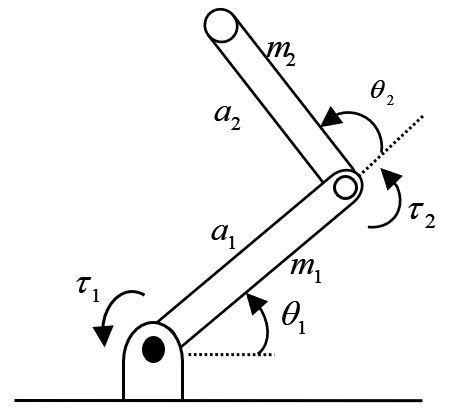
To verify the effectiveness of the proposed method, a two link robot manipulator with two Revolute joints (RR) shown in Figure 4 will be considered.
Figure 4. Two link planar RR arm
The dynamic of the two link robot is defined by Eq. (1) for which we will use the following parameters:
Masse matrix
$H\left( q \right)=\left[ \begin{matrix} {{h}_{11}} & {{h}_{12}} \\ {{h}_{21}} & {{h}_{22}} \\\end{matrix} \right]$
${{h}_{11}}=\left( {{m}_{1}}+{{m}_{2}} \right)a_{1}^{2}+{{m}_{2}}a_{2}^{2}+2{{m}_{2}}{{a}_{1}}{{a}_{2}}\cos {{\theta }_{2}}$
${{h}_{12}}={{h}_{21}}={{m}_{2}}a_{2}^{2}+{{m}_{2}}{{a}_{1}}{{a}_{2}}\cos {{\theta }_{2}}$
${{h}_{22}}={{m}_{2}}a_{2}^{2}$
The parameters ${{m}_{i}}$ and ${{a}_{i}},(i=1,2)$ are the masses and lengths of the robot manipulator.
Centrifugal and coriolis forces matrix
$C\left( q,\dot{q} \right)=\left[ \begin{matrix} -2{{m}_{2}}{{a}_{1}}{{a}_{2}}{{{\dot{\theta }}}_{2}}\sin {{\theta }_{2}} & -{{m}_{2}}{{a}_{1}}{{a}_{2}}{{{\dot{\theta }}}_{2}}\sin {{\theta }_{2}} \\ {{m}_{2}}{{a}_{1}}{{a}_{2}}{{{\dot{\theta }}}_{1}}\sin {{\theta }_{2}} & 0 \\\end{matrix} \right]$
Gravitational forces matrix
$g\left( q \right)=\left[ \begin{matrix} \left( {{m}_{1}}+{{m}_{2}} \right)g{{a}_{1}}\cos {{\theta }_{1}}+{{m}_{2}}g{{a}_{2}}\cos \left( {{\theta }_{1}}+{{\theta }_{2}} \right) \\ {{m}_{2}}g{{a}_{2}}\cos \left( {{\theta }_{1}}+{{\theta }_{2}} \right) \\\end{matrix} \right]$
with $g=9.8m/{{s}^{2}}$ is the acceleration due to gravity.
For simulation purposes we take ${{m}_{1}}={{m}_{2}}=1\,kg$ and ${{a}_{1}}={{a}_{2}}=1\,m$. Since the dynamic of the considered system is two dimensional, therefore the joint variable and the generalized force vector will be defined by $q={{\left[ \begin{matrix} {{\theta }_{1}} & {{\theta }_{2}} \\\end{matrix} \right]}^{T}}$ and $\tau ={{\left[ \begin{matrix} {{\tau }_{1}} & {{\tau }_{2}} \\\end{matrix} \right]}^{T}}$, respectively, with ${{\tau }_{1}}$ and ${{\tau }_{2}}$ are the torques supplied by the actuators. Note that all of our codes are written in Matlab language in M-files with sampling period ${{10}^{-3}}\,s$. For comparison purposes, the optimization performances are evaluated using the MAE criterion.
In fact, it is not simple to deduce exact values for ${{K}_{p}}$, ${{K}_{i}}$ and ${{K}_{d}}$ giving the best performances. This will be solved in what follows by using our PSO-PD and PSO-PID which will allow us to obtain better results with higher precision than the classical trial and error method. It should be noted that the convergence of the PSO method to the optimal solution depends on the parameters ${{c}_{1}}$, ${{c}_{2}}$ and $w$. According to our tests, ${{c}_{1}}$ and ${{c}_{2}}$ best values lie in the interval [0.5, 1.05]; and $w\in \left[ 0.3,1 \right]$.
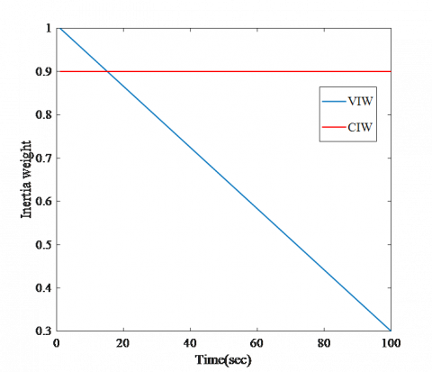
In this paper, two strategies are used for the computation of the inertia weight $w$to evaluate the performance of parameters. The inertia weight $w$is introduced into the equation to balance between the capacities of the global search and the local search, as it is one of the important factors for the PSO’s convergence which directly affects the percentage of previous velocities on the current velocity at the current time step for both strategies: (1) PSO with Constant Inertia Weight (PSOCIW), in which it will be fixed at 0.9 (see Figure 5), this high value of $w$ will force the particles to fly with a significant influence of the previous velocity. Note that this method is characterized by an increase in the convergence speed of the PSO algorithm and a large inertia weight factor provides PSO a global optimum. (2) PSO with Variable Inertia Weight (PSOVIW) was introduced in PSO’s equations in order to improve the performance of PSO (according to Eq. (20)), in which it will be decreased linearly with the iteration number (see Figure 5) to a small value. With this low value of $w$, current velocity will contribute more to the particle’s trajectory and provides PSO a local optimum, in contrast to the first strategy. For high values of inertia weight, the global search capability is powerful but the local search capability is powerless. Likewise, when inertia weight is lower, the local search capability is powerful, and the global search capability is powerless. This balancing improves the performance of PSO.
${{w}_{k}}={{w}_{\max }}-\frac{{{w}_{\max }}-{{w}_{\min }}}{N}k$ (20)
where, ${{w}_{\max }}=1$ and ${{w}_{\min }}=0.3$ are the initial and final values of the inertia weight, respectively, and $N$ is the maximum number of iterations used in PSO.
Note that, in this case, excellent results will be obtained as will be shown later.
The PSO Parameters of the two strategies PSOCIW and PSOVIW are summarized in Tables 1 and 2.
The best fitness functions (MAEs) and their corresponding optimized controllers gain parameters $\left( {{K}_{p}}\,\,,{{K}_{i}}\,and\,{{K}_{d}} \right)$ obtained by our proposed approaches (combination PSO-PD and PSO-PID) (see Figure 3) are reported in Table 3 and Table 4, respectively.
Figure 5. CIW and VIW of PSO algorithm
Table 1. Parameters of the PSOCIW algorithm
|
Designation |
Variable |
Value |
|
Number of particles in a group |
N |
20 |
|
Number of Iterations |
I |
40, 50, 60, 100 |
|
Inertia weight factor |
w |
0.9 |
|
Acceleration constants |
c1, c2 |
0.5 |
Optimization results show that the method is able to find the optimal solution and reduce the error efficiently within 100 iterations. We note that the best value of MAE which corresponds to the best estimate of PD and PID gain parameters are given in case 8 of Table 3 and case 7 of Table 4, respectively.
Table 2. Parameters of the PSOVIW algorithm
|
Designation |
Variable |
Value |
|
|
Number of particles in a group |
N |
20 |
|
|
Number of Iterations |
I |
40, 50, 60, 100 |
|
|
Minimum inertia weight factor |
wmin |
0.3 |
|
|
Maximum inertia weight factor |
wmax |
1 |
|
|
Acceleration constants |
c1, c2 |
1.05 |
|
Table 3. Optimized parameters and their performances in the joint space for PD controller using PSO
|
Optimization method |
Case |
I |
Kp1 |
Kd1 |
Kp2 |
Kd2 |
MAE |
|
PSOCIW |
1 2 3 4 |
40 50 60 100 |
553.5999 556.1911 558.1911 558.1911 |
88.3948 87.0808 87.0808 87.0808 |
376.4420 369.5691 369.5691 369.5691 |
37.3761 31.2962 31.2962 31.2962 |
1.0737e-05 9.7914e-06 1.3111e-06 1.3111e-06 |
|
PSOVIW |
5 6 7 8 |
40 50 60 100 |
521.1328 597.0536 816.1067 663.2064 |
51.3526 62.0977 89.9357 113.7360 |
544.2311 560.3582 418.7053 695.1595 |
75.9123 67.0380 43.7568 105.5423 |
6.6234e-06 1.5341e-06 6.0632e-10 1.5916e-14 |
Table 4. Optimized parameters and their performances in the joint space for PID controller using PSO
|
Optimization method |
Case |
I |
Kp1 |
Ki1 |
Kd1 |
Kp2 |
Ki2 |
Kd2 |
MAE |
|
PSOCIW |
1 2 3 4 |
40 50 60 100 |
575.8960 575.8960 575.8960 577.0524 |
392.3983 392.3983 392.3983 356.7020 |
112.5328 112.5328 112.5328 105.4120 |
392.4810 392.4810 392.4810 344.7770 |
462.4569 462.4569 462.4569 432.3530 |
9.5001 9.5001 9.5001 10.1167 |
1.8169e-04 1.8169e-04 1.8169e-04 1.3856e-05 |
|
PSOVIW |
5 6 7 8 |
40 50 60 100 |
417.6209 509.3163 435.5346 426.8821 |
123.9084 181.1770 100.8813 124.1054 |
71.2909 65.0094 56.4018 76.5055 |
644.9327 775.7143 621.7791 641.5470 |
625.4555 661.6406 517.8345 546.7384 |
79.8841 73.8510 59.1068 83.0836 |
3.7550e-18 3.0524e-18 3.7466e-19 1.1656e-18 |
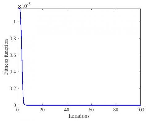
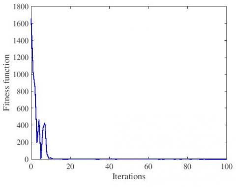
Figure 6. Evolution of the fitness function relative to PD (case of 8 iterations in Table 3)
Figure 7. Evolution of the fitness function relative to PID (case of 8 iterations in Table 4)
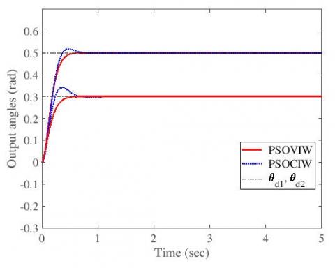
(a) Constant desired trajectory
(b) Sinusoidal desired trajectory
Figure 8. PD Positions tracking with the best optimized parameters
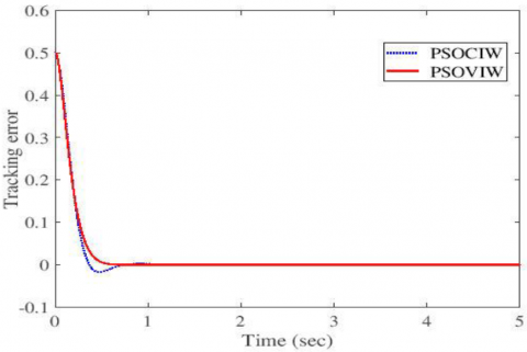
Figure 9. Tracking position error ${{e}_{1}}$ of the first articulation
Figure 10. Input control action ${{u}_{1}}$ of the first articulation
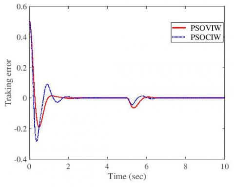
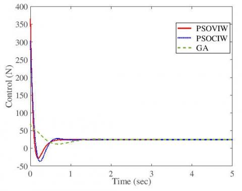
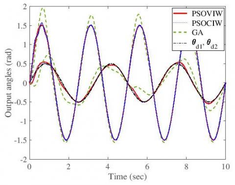
Same interpretation for PID controller (see Figure 11) in which we visualize also an excellent perturbation rejection.
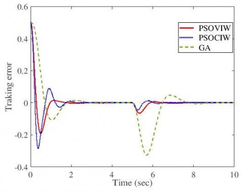
Note that the perturbation was applied at t=5s with amplitude 5N. The corresponding tracking error and control action relative to the first articulation of the robot are presented in Figures 12 and 13 where we denote perfect performances.
(a) Constant desired trajectory
(b) Sinusoidal desired trajectory
Figure 11. PID Positions tracking and perturbation rejection with the best optimized parameters
Figure 12. Tracking position error ${{e}_{1}}$ of the first articulation
Figure 13. Input control action ${{u}_{1}}$ of the first articulation
The convergence of the fitness functions is shown in Figures 6 and 7 for PD and PID controllers; respectively. We notice that the MAE is decreased at most after 10 iterations, which confirms the convergence and the stability of the optimization process.
Simulation results for the PD controller are given in Figure 8 where we show that the performances of PSOVIW are better than PSOCIW for both cases: constant desired trajectory (Figure 8 (a)) and sinusoidal desired trajectory (Figure 8 (b)). We also present in Figures 9 and 10 the corresponding tracking error and control action of the first articulation. Remark that the tracking error converges exponentially to zero.
To validate the proposed approach, we will present in what follows a short comparative study in which we compare the introduced method with Genetic Algorithm.
Genetic Algorithm will play now the same role as PSO, which means that we replace in Figure 3 the PSO block by a GA block. For this purpose, GA will estimate and optimize the controller parameters in two steps as in the case of PSO.
The parameters of GA are chosen as shown in Table 5 where we have selected different generations I=40, 50, 60, 100 with the following parameters: population size N=20, mutation probability M=0.2 and crossover probability C= 0.5.
GA fitness functions evolution are presented in Figures 14 and 15 for PD and PID controllers; respectively. We notice that the MAE converges in 20 iterations max, contrary to the PSO case which converges in 10 iterations max (see Figures 6, 7, 14 and 15) which confirm that PSO is faster than GA. Note also that both PSO methods (PSOCIW and PSOVIW) give more accurate results compared to GA method (See Tables 3, 6 and Tables 4, 7).
By this short comparative study, we confirm the effectiveness of the proposed method and its superiority in speed convergence high resolution (see Figures 16-21).
Table 5. Parameters of the genetic algorithm
|
Designation |
Variable |
Value |
|
Population size |
N |
20 |
|
Generations |
I |
40,50,60,100 |
|
Mutation probability |
M |
0.2 |
|
Crossover probability |
C |
0.5 |
Table 6. Optimized parameters and their performances in the joint space for PD controller using GA
|
Optimization method |
Case |
I |
Kp1 |
Kd1 |
Kp2 |
Kd2 |
MAE |
|
GA |
1 2 3 4 |
40 50 60 100 |
64.6040 76.2287 52.9399 89.0021 |
28.6951 30.2603 23.6698 30.7783 |
46.9204 74.9499 79.5247 49.2828 |
10.1212 13.9796 14.4101 1.3190 |
1.8757e-04 6.3897e-05 9.3264e-05 9.9626e-05 |
Table 7. Optimized parameters and their performances in the joint space for PID controller using GA
|
Optimization method |
Case |
I |
Kp1 |
Ki1 |
Kd1 |
Kp2 |
Ki2 |
Kd2 |
MAE |
|
GA |
1 2 3 4 |
40 50 60 100 |
45.9883 77.2967 77.6165 110.8116 |
3.7957 7.7502 7.5343 15.3839 |
23.2161 30.5331 32.2968 33.3837 |
44.7578 64.3610 87.5616 75.5687 |
10.5608 49.7162 19.1396 22.9882 |
2.2023 5.1843 3.1810 3.9823 |
1.0940e-03 3.3240e-03 8.7338e-04 1.5665e-04 |
Figure 14. Evolution of the fitness relative to PD (case 4 iterations in Table 6)
Figure 15. Evolution of the fitness relative to PID (case 4 iterations in Table 7)
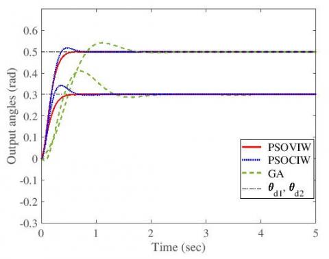
(a) Constant desired trajectory
(b) Sinusoidal desired trajectory
Figure 16. PD Positions tracking with the best optimized parameters
Figure 17. Tracking position error ${{e}_{1}}$ of the first articulation
Figure 18. Input control action ${{u}_{1}}$ of the first articulation
(a) Constant desired trajectory
(b) Sinusoidal desired trajectory
Figure 19. PID Positions tracking and perturbation rejection with the best optimized parameters
Figure 20. Tracking position error ${{e}_{1}}$ of the first articulation
Figure 21. Input control action ${{u}_{1}}$ of the first articulation
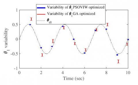
To confirm the efficiency of the proposed control, we present in the following a statistical comparison between the best obtained results of PSOVIW and GA for PID case. As a statistical analysis tool, we are going to use the error bars for the optimized parameters to evaluate the accuracy of the control quality. This technique is a graphical representation of the variability of the optimized parameters (on graphs) to indicate the uncertainty and provides a general idea of the tracking precision. If the bars are large, this means we have bad optimization (high variability or high uncertainty), contrary, if the bars are narrow, then the optimization quality is better (less uncertainty).
We present in Figures 22 and 23 error bars comparison between the PSOVIW and GA of the first and the second joints of the robot using the best parameters given in the last line in Table 4 for PSOVIW case and the best parameters given in the last line in Table 7 for GA case. For this purpose, we introduce state random noise $n(t)$ with variance one and mean value zero i.e., $n(t)\sim N(0,1)$. Figures 22 and 23 suggest clearly that widths of the error bars for the PSOVIW method are the narrowest and more centered compared to the GA case. Error bars in Figures 22 and 23 confirm the efficiency of PSOVIW method compared to GA method where we notice that PSOVIW tracking variance is tighter and well centered.
Figure 22. Error bar comparison of tracking variability of the first joint
Figure 23. Error bar comparison of tracking variability of the second joint
In this paper, we proposed a metaheuristic optimization method using Particle Swarm Optimization for the adjustment of PD and PID gains. Two PSO approaches were used: PSOCIW and PSOVIW. In this technique, the algorithms were combined with PID and PD controllers for the purpose of improving controller effectiveness. The approaches were designed to estimate offline controller parameters. After that, optimal estimated parameters were injected in the online control loop. The introduced algorithms were validated on the control of a two link robot manipulator. Simulation results show that the method gives an excellent performance. Also, the effectiveness of the approach was confirmed by a short comparative study in which we found that it outperforms the Genetic Algorithm technique for this type of applications, where the resulting estimates are more precise and the optimization is faster than GA. Furthermore, we concluded that the PSOVIW approach, which used variable inertia weight, performed better results than GA and PSOCIW.
[1] Jaleel, J.A., Thanvy, N. (2013). A comparative study between PI, PD, PID and lead-lag controllers for power system stabilizer. IEEE Trans. International Conference on Circuits, Power and Computing Technologies [ICCPCT], pp. 456-460. http://dx.doi.org/10.1109/ICCPCT.2013.6528877
[2] Fadil, M.A., Darus, I.Z. (2013). Evolutionary algorithms for self-tuning active vibration control of flexible beam. Engineers Australia. Australian Control Conference, pp. 104-108. http://dx.doi.org/10.1109/AUCC.2013.6697256
[3] Kecskes, I., Odry, P. (2014). Optimization of PI and fuzzy-PI controllers on simulation model of szabad(ka)- II walking robot. International Journal Advanced Robotic Systems, 11(11): 186. http://dx.doi.org/10.5772/59102
[4] Mahmoodabadi, M.J., Momennejad, S., Bagheri, A. (2014). Online optimal decoupled sliding mode control based on moving Least squares and particle swarm optimization. Information Sciences, 268: 342-356. http://dx.doi.org/10.1016/j.ins.2014.01.027
[5] Khong, S.Z., Tan, Y., Manzie, C., Nešić, D. (2015). Extremum seeking of dynamical systems via gradient descent and stochastic approximation methods. Automatica, 56: 44-52. http://dx.doi.org/10.1016/j.automatica.2015.03.018
[6] Kumar, S., Gaur, P. (2015). Comparative response of filter using GA PSO BBO. International Journal Advanced Research in Computer and Communication Engineering, 4(8): 83-86. http://dx.doi.org/10.17148/IJARCCE.2015.4816
[7] Pano, V., Ouyang, P.R. (2014). Comparative study of GA, PSO, and DE for tuning position domain PID. Prod of IEEE. International Conference on Robotics and Biomimetics, pp. 1254-1259. http://dx.doi.org/10.1109/ROBIO.2014.7090505
[8] Bechouat, M., Soufi, Y., Sedraoui, M., Kahla, S. (2015). Energy storage based on maximum power point tracking in photovoltaic systems: A comparison between GAs and PSO approaches. International Journal Hydrogen Energy, 40(39): 13737-13748. http://dx.doi.org/10.1016/j.ijhydene.2015.05.008
[9] Sharma, R., Rana, K.P.S., Kumar, V. (2014). Statistical analysis of GA based PID controller optimization for robotic manipulator. IEEE Trans. International Conference Issues and Challenges in Intelligent Computing Techniques (ICICT), pp. 713-718. https://doi.org/10.1109/ICICICT.2014.6781368
[10] Kennedy, J., Eberhart, R. (1995). Particle swarm optimization. IEEE Trans. International Conference on Neural Networks, pp. 1942-1948. http://dx.doi.org/10.1109/ICNN.1995.488968
[11] Shen, Y., Wang, G., Tea, C. (2011). Particle swarm optimization with novel processing strategy and its application. International Journal Computational Intelligence Systems, 4(1). http://dx.doi.org/10.2991/ijcis.2011.4.1.9
[12] Laamari, Y., Chafaa, K., Athamena, B. (2015). Particle swarm optimization of an extended Kalman filter for speed and rotor flux estimation of an induction motor drive. Electrical Engineering, 97(2): 129-138. http://dx.doi.org/10.1007/s00202-014-0322-1
[13] Aftab, M., Shadab, M., Santosh, P., Taili, J. (2013). Optimal control of multi-axis robotic system using particle swarm optimization. Annual IEEE India Conference (INDICON). http://dx.doi.org/10.1109/INDCON.2013.6726104
[14] Luchi, F., Krohling, R.A. (2015). Differential evolution and nelder-mead for constrained non-linear optimization problems. Procedia Computer Science, 55: 668-677. http://dx.doi.org/10.1016/j.procs.2015.07.071
[15] Mohanty, B., Panda, S., Hota, P.K. (2014). Differential evolution algorithm based automatic generation control for interconnected power systems with non-linearity. Alexandria Engineering Journal, 53(3): 537-552. http://dx.doi.org/10.1016/j.aej.2014.06.006
[16] Mohanty, B., Panda, S., Hota, P.K. (2014). Controller parameters tuning of differential evolution algorithm and its application to load frequency control of multi-source power system. Electrical Power and Energy Systems, 54: 77-85. http://dx.doi.org/10.1016/j.ijepes.2013.06.029
[17] Tripathi, S., Shrivastava, A., Jana, K.C. (2020). GWO based PID controller optimization for robotic manipulator. Intelligent Computing Techniques for Smart Energy Systems, 943-951. http://dx.doi.org/10.1007/978-981-15-0214-9_100
[18] Nedjah, N., De, M.M. (2006). Swarm Intelligent Systems. Springer-Verlag, Berlin Heidelberg. http://dx.doi.org/10.1007/978-3-540-33869-7
[19] Parsopoulos, K.E., Vrahatis, M.N. (2004). On the computation of all global minimizers through particle swarm optimization. IEEE Transactions on Evolutionary Computation, 8(3): 211-224. http://dx.doi.org/10.1109/TEVC.2004.826076
[20] Vastrakar, N.K., Padhy, P.K. (2013). Simplified PSO PI-PD controller for unstable processes. 4th International Conference on Intelligent Systems, Modeling and Simulation, pp. 350-354. http://dx.doi.org/10.1109/ISMS.2013.133
[21] Taeib, A., Ltaief, A., Chaari, A. (2013). PID control based on modified particle swarm optimization for nonlinear process. World Congress on Computer and Information Technology (WCCIT), IEEE, pp. 1-5. http://dx.doi.org/10.1109/WCCIT.2013.6618723
[22] Huang, Y.C., Su, Y.W. (2014). Study on iterative learning control bandwidth tuning using particle swarm optimization technique for high precision motion. International Conference on Information Science, Electronics and Electrical Engineering, IEEE, pp. 2033-2037. http://dx.doi.org/10.1109/InfoSEEE.2014.6946280
[23] Fan, X., Cao, J., Yang, H., Dong, X., Liu, C., Gong, Z., Wu, Q. (2013). Optimization of PID parameters based on improved particle swarm optimization. International Conference on Information Science and Cloud Computing Companion, pp. 393-397. http://dx.doi.org/10.1109/ISCC-C.2013.99
[24] Meng, M.Q.H. (1992). Model based adaptive position and force control of robot manipulators. Proquest Dissertations and Theses. http://hdl.handle.net/1828/9585.
[25] Lazinica, A. (2009). Particle Swarm Optimization. In-Tech, Croatia. http://dx.doi.org/10.5772/109