Abdelouadoud Loukriz* | Djamel Saigaa | Mahmoud Drif | Moufdi Hadjab | Azeddine Houari | Sabir Messalti | Mohammad Alam Saeed
© 2021 IIETA. This article is published by IIETA and is licensed under the CC BY 4.0 license (http://creativecommons.org/licenses/by/4.0/).
OPEN ACCESS
This paper proposes a generalized technique to minimize power losses of PV arrays connected in Total Cross-Tied (TCT), under both current and voltage mismatch effects. The proposed method is based on the classification of the electrical data of the PV modules composing the photovoltaic array in order to identify the mismatch type, then applying an arrangement of the PV modules according to the mismatch type found. The design process of the proposed algorithm is detailed and its validity and performance are verified under different mismatch scenarios. The efficiency enhancement is verified for different mismaths cases and the computed results reveal that the proposed algorithm can achieve an improvement of around 30% in the PV array power. Furthermore, a comparative study with SuDoKu and genetic algorithms are performed. The obtained results under MATLAB/Simulink software highlighted the superiority of the proposed method in comparison to the compared ones. The enhancement resides in the implementation simplicity as well as in the minimization of the number of infection points indicating smooth I-V and P-V characteristic curves.
current mismatch, PV array reconfiguration, parallel resistance, PV module aging. simplified algorithm, Serie resistance, temperature variation, voltage mismatch
In a world where the environment faces threats from pollution and the greenhouse effect, the production of electricity by clean means has become an essential necessity [1]. Solar photovoltaic (PV) represents a clean and non-exhaustive energy source [2]. It is a vital component of renewable energy which can help the world to meet its ever-growing energy needs, as well as limit the increasing emissions of greenhouse gases and reduce environmental pollution [1, 3, 4]. According to the latest statistics from the International Energy Agency (IEA), solar photovoltaic production increased by 22% (+131 TWh) with the second highest absolute production growth of all renewable technologies, slightly behind wind power and ahead of hydroelectricity [5]. In other words, the photovoltaic is an intermittent energy. It is an interesting solution as an alternative or complement to conventional sources of electricity production, due to its many advantages such as the electricity production of the free and renewable energy of the sun with no fuel requirement, a medium reliability that is low in maintenance, it is silent, clean and environmentally friendly [6-8]. However, the PV system efficiency is subject to various factors such as working condition changes (solar radiation, temperature, dust, shade) and ageing. These effects become serious challenges that deteriorate the PV system output power since the PV array is composed of interconnected PV modules that can have different conditions [9]. As result, the efficiency decreases due to mismatch losses [10, 11].
Indeed, interconnections of solar cells (or modules) that do not have the same properties or that are under different meteorological conditions from one another yield to a deteriorated efficiency. In practice, mismatch issue, is reflected reduction of the current or/and the voltage of the concerned module [12, 13]. Another key point to remember, the partial shading is just a part of mismatch issue and is not the only phenomenon influencing power generation. The temperature of the solar cells is a very important parameter that cannot be neglected in the behaviour of solar modules [14, 15]. During the last few years, the number of installed PV modules has been increasing significantly. The estimated lifetime of PV modules is around 25 years. During this time, the PV modules suffer degradation caused by exposure to solar radiation, humidity and temperature difference [16]. The ambient temperature variation and the ageing of the PV modules strongly influence the electrical parameters [17]. During parallel connection of PV modules under non-homogeneity, the affected modules PV force the healthy modules to operate in the negative voltage area and results in a net loss of the voltage in the system. The affected modules absorb the power and begin to act as a load. In other words, affected modules PV dissipate power as heat and cause hot spots [18]. To deal with, many studies based on reconfiguring the solar PV modules have been carried in literature [19-24]. The reconfiguration of solar PV arrays is a well-known and a widely used method to increase the power output and production efficiency of power generation. The conventional configuration type of a solar PV system can be categorized into four types: serial-parallel (SP), HC (honey-comb), bridge-linked (BL), and total cross-tied (TCT). In case of the SP, this type of configuration is a combined series and parallel connection of every module. In BL, HC, the connection of every module is similar to the SP configuration, but the connections of certain lines within each chain are added. Lastly, in TCT, the connection of every module is almost the same as in BL, except there are connections for all the lines between each string. The TCT configuration is mostly adequate to minimize operating losses when a PV array is under shade [19].
To deal with, in this paper a generalized technique to minimize power losses of PV arrays is proposed. This method is based on the classification of the electrical data of the PV modules composing the photovoltaic array in order to identify the mismatch type, then applying an arrangement of the PV modules according to the mismatch type found. The main contributions of this paper are listed below:
- New method has been proposed and investigated.
- The proposed approach provides a better output power in any mismatch conditions.
- Comparative study with TCT, SuDoKu, and GA methods.
- Proposing a simple, fast and accurate algorithm, with absolute precision. It can easily be coded in any machine language, with real-time execution and without heavy computation.
- The reconfiguration is based on the electrical reallocation of PV modules which is initially interconnected in TCT, while keeping the physical location of the PV modules unchanged (no more wiring).
- Provides a better energy harvest in any mismatch conditions (shading, temperature, aging…).
- Additionally to the improved output power, the shapes of the I-V and P-V curves obtained are smooth with a minimum number of infection points (local minimum), this important contribution will facilitate the finding of the global power point (GMPP) by the MPPT controller.
To validate the proposed algorithm, several mismatch scenarios have been applied on a solar PV system. For further validation, a comparative investigation with the GA genetic algorithm is also carried out. MATLAB /Simulink software is used for simulation.
The rest of this paper is arranged as follows. Section 2 summarizes the related works on adaptive reconfiguration of solar array connections techniques. However, in section 3 describes the electric characteristics of a PV solar cell. Section 4, present the PV solar array mismatch losses. In section 5, the proposed algorithm is described in detail. In section 6, the performance assessment of the proposed method in comparison with TCT, SuDoKu and GA reconfiguration techniques are presented. In addition, the obtained results from the comparative simulation study are highlighted and discussed in this section. Section 7, summarizes the main conclusions of the presented work.
Different studies are performed to evaluate the different cited configurations. In 2009 Ramaprabha and Mathur studied the impact of the shading in solar PV array under a series configuration [20]; employing a software simulation in MATLAB using MPPT method. The results indicate that a shaded module behaves like an electrical load and can be affected by heat accumulation. To protect solar PV module against such damage, they have used bypass diodes, the main inconvenience is to have many local maximums in the output signal, which implies a difficulty to follow the point of maximum output power. In 2011, Buddha [21] studied the PV array configuration by utilizing 52 PV solar panels which were placed in an array of 13×4. The effectiveness of the conventional configuration was tested and confirmed. If parts of PV modules are shaded, the power output varies according to the number of shaded modules. The SP configuration can produce the maximum output at low shaded areas. Therefore, the TCT configuration can offer the maximum output, which is 5% higher than the SP, at higher shaded areas. In 2013, Rani et al. [22] proposed a new method of reconfiguring the PV modules interconnected in TCT, the approach based on the Su Do Ku puzzle patterns to distribute the shading effect over the entire array. A solar system of 81 PV modules (9×9) interconnected in TCT was studied using the proposed approach, under different shading scenarios and an improvement up to 26% especially in the first case studied (short wide) was found. However, in other cases, the power enhancement was 3.6% to 20.5%. In 2015, Deshkar et al. [23] presented a reconfiguration of 81 PV modules placed on 9 × 9 modules and interconnected in TCT via MATLAB/Simulink. The solar irradiation varied between 200 and 900 W/m2. The genetic algorithm (GA) has been utilized for finding an ideal reconfiguration for every shadow in order to achieve the maximal output power. This study found that the GA provided 34.96% more power than a fixed TCT configuration. It is noted that this algorithm has been tested for only one mismatch issue (shading).
There are many studies explaining the methods of reconfiguration that minimize the impact of shading on the solar photovoltaic array as much as possible. To find a suitable reconfiguration method, mathematical methods, relocation methods and meta-heuristic methods, like GA, and Particle Swarm Optimization (PSO) were used [24].
The cited methods above allow increasing the efficiency of PV installations. However, it’s worth to be mentioned that each method has its own limitation, specifically regarding to the mismatch origins. For instance, with methods based on dynamic reallocation of PV modules, the following points may be underlined:
-Need for high-speed processing and high working memory capacity.
-Need for a larger adaptive bank to respond to all possible types of shadows, which increases the cost of the system considerably.
-Only treats the phenomenon of shading.
For methods of physical reallocation of PV modules:
-Low shadow dispersion.
-A complexity of wiring.
-Treated the phenomenon of shading only.
In the last years, the PV modules suffer degradation caused by exposure to solar radiation, humidity and temperature difference. En consequence, the Potential Induced Degradation (PID) loss in solar cells and the other failures like diode failure, cells interconnect failure breakage are affected the PV array installation. Those failures influence in the voltage output of the PV modules. Therefore, it makes a voltage mismatch between the PV modules constitute the PV array. In this respect, the authors have proposed a new approach to deal with the voltage and current mismatch phenomena affecting the PV array.
A photovoltaic solar cell is characterized by its current-voltage curve, which is divided into four quadrants. However, the behaviour of the PV cell extends over three zones (I, II and IV) and depends on its polarization condition, as shown in the Figure 1. However, zone I (I > 0, V > 0) corresponds to generator operation. If the current flowing through the cell, due to the external circuit, exceeds the value of the short-circuit current (zone II), the cell works as a receiver, with a very high impedance, like a reverse-biased diode. If the voltage across the cell exceeds Voc (zone IV), the cell will work as a receiver again, but this time with very low impedance, like a forward biased diode. We observe that in zones II and IV, the solar cell behaves as a receiver by dissipating energy. It is therefore important to prohibit its operation in these two zones to avoid destruction. However, in Zone I, the solar cell works as a generator by providing power. Idealistically, it is desired operation to keep it in this area of operation [25, 26].
Figure 1. I-V characteristics with the operation mode in each
Mismatch losses result from the interconnection of PV solar cells or PV modules are either in series or parallel. The mismatch losses are a serious issue in PV modules and arrays because this causes a drop in output power, reducing the efficiency and performance of the system. Indeed, in the worst case, the efficiency of the whole PV array is determined by the solar module with the lowest efficiency. As an example, when one PV module is shaded and the other modules are not, the power generated by the "good" modules may be dissipated by the worst performing module rather than being used to supply the load. In turn can lead to very localized power dissipation and resulting local heating can cause irreversible damage to the PV module. The mismatch problem can be categorized into two classes [27, 28]:
- Voltage mismatch: it is due to the temperature variation of one or more PV modules, or a reduction in the parallel resistance value caused by the ageing of the PV modules.
- Current mismatch: it is due to shading of the PV modules or an increase in series resistance due to the ageing phenomenon.
The mismatch in the parallel connection is found in the large array of PV solar module. Voltage mismatch is occurring when strings with different voltage (measured independently) are interconnected and, as a result, the total installation is operating at a voltage equivalent to that of the worst performing string (leading to power output losses). However, a more serious problem is encountered when there is a large voltage mismatch between strings interconnected in parallel. Due to this strong mismatch, the modules start operating at a point far from their Maximum Power Point (MPP). This operation, in addition to the power loss, causes inverter to operate longer outside its ideal voltage range, which affects the efficiency of the power inverter.
4.1 PV Cells or modules connected in parallel without a mismatch issue
$I_{T}=I_{1}+I_{2}$ (1)
$V_{T}=V_{1}=V_{2}$ (2)
Figure 2. PV cells in parallel connection without a mismatch issue
A case of modules connected in parallel without any mismatch problems is shown in Figure 2. In this case, the terminal voltage of combination of modules is always same, while the total current of the combination is the sum of the currents in the individual modules [27].
4.2 PV Cells or modules connected in parallel with the mismatch issues
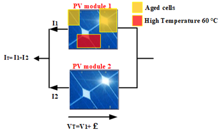
Figure 3. PV cells in parallel connection with a voltage mismatch
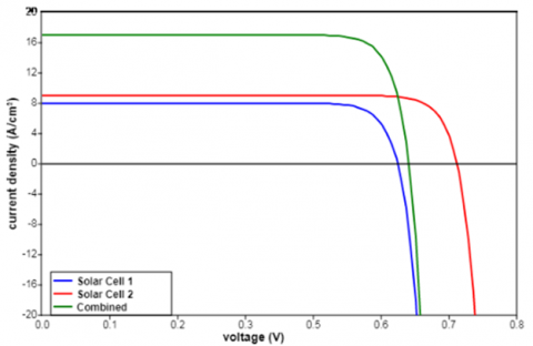
Figure 4. I-V curve example of two PV cells connected in parallel with a voltage mismatch
Figure 3 shows two cells connected in parallel with a voltage drop in the first cell due to ageing or an increase in the ambient temperature. The affected PV cell or module has started to dissipate power from the other cells or modules connected in parallel, due to its operation in zone IV, as mentioned in the previous section (II). Therefore, the voltage mismatches for two modules in parallel, as shown in the Figure 4. The individual modules are shown in red and blue and the green curve indicates the IV curve of combination.
In the current axis, the combined current is the sum of the individual current. Therefore, in the voltage axis, the resulting voltage was led by the lowest voltage module (blue curve), as discussed in the previous section, when the voltage across the cell exceeds Voc due to the parallel module (red curve), the lowest voltage module (blue curve) begins working in the zone IV as a load with very low impedance, resulting a progressive dissipation of the combined output voltage (green curve). The combination voltage is between the voltages of the individual modules [27].
However:
$V_{\alpha 1}<V_{\alpha 2}$ (3)
$V_{T}=V_{\alpha 1}+\zeta$ where $I_{T}=0$ (4)
$I_{T}=I_{1}+I_{2}$ (5)
$P_{T}=V_{T} \times I_{T}$ (6)
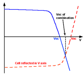
Figure 5. A graphical way to calculate the combined voltage
The terminal voltage can be measured by an easy method of calculating the combined open circuit voltage (Voc) of mismatched modules connected in parallel (Figure 5). The curve for the higher voltage of modules is reflected in the voltage axis, so that the intersection point between curves of the higher and lower voltage is the voltage of the parallel configuration (at I1+I2=0) [27].
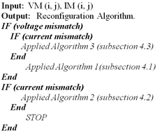
The output power is optimized by minimizing the losses due to different types of mismatches between the PV modules. A simple algorithm is proposed (See Figure 6) which has the possibility to reconfigure the PV modules according to the type of existing mismatch. In the first step, and after having the database of voltage and current values of each PV module, we classify the mismatch to choose an appropriate algorithm. In the case of the voltage, we apply the voltage balancing algorithms. Otherwise, for the current mismatch type, the row current balancing algorithm is used. If the mismatch problem is hybrid (voltage and current), the power balancing algorithm is applied. In the following section, we will provide a descriptive detail about the employed algorithms.
Figure 6. The Pseudo code for proposed reconfiguration technique
5.1 Voltage-Balancing algorithm
Figure 7. Main steps of the voltage balancing algorithm
The PV array under voltage mismatch conditions has a better power output when the affected modules are grouped in the same row, or in a limited number of rows. Figure 7 shows the principle of balancing algorithm based on measuring the output voltages of each PV module. The first step is to extract the voltage values of each PV module of PV array by putting the data into a matrix (n×m). This voltage matrix is then converted into a state vector. These voltages are then sorted according to their values in an increasing order. The vector of the numerical values of voltages is then truncated on the number of columns n of the data matrix to obtain m lines of values of nearby parallel voltages. Then this combination is injected into the truth table where it is defined in the state of switches to be piloted. As illustrated in Algorithm 1, a simple method used to reconfigure the PV array under voltage mismatch conditions.
$\begin{align} & A\lg orithm\text{ }1\text{ }:\,Voltages\text{ }Balancing \\ & \_\_\_\_\_\_\_\_\_\_\_\_\_\_\_\_\_\_\_\_\_\_\_\_\_\_\_\_ \\ & \\ & INPUT:\,\,{{V}_{out}}\,,\,{{V}_{pilot}} \\ & \\ & OUTPUT\,:V{{M}_{NEW}}(i,j)\,\,New\,Voltages\,Matrix\, \\ & 1-Filling\text{ }of\text{ }the\text{ }voltages\text{ }matrix\text{ }VM(i,j)\,. \\ & 2\,-\,Converting\text{ }the\text{ }voltages\text{ }matrix\text{ }VM(i,j)\text{ }to\text{ }a\text{ }state\text{ }vector\,A(k)\,. \\ & For\,i=1\,to\,n\,do \\ & \,\,\,\,\,\,\,\,\,For\,j=1\,to\,m\,do \\ & \,\,\,\,\,\,\,\,\,\,A(k)=VM(i,j) \\ & \,\,\,\,\,\,\,\,\,\,\,k=k+1 \\ & \,\,\,\,\,\,\,\,\,\,End\,For \\ & End\,For \\ & 3-\,Sort\text{ }the\text{ }voltages\text{ }values\,of\,A(k)\text{ }from\text{ }l\arg est\text{ }to\text{ }smallest. \\ & For\,i=1\,to\,n\times m-1\,do \\ & \,\,\,\,\,\,\,\,\,For\,j=i+1\,to\,n\times m\,do \\ & \,\,\,\,\,\,\,\,\,\,\,\,\,\,\,\,\,\,if\,A(i)>A(j)\,Then\, \\ & \,\,\,\,\,\,\,\,\,\,\,\,\,\,\,\,\,\,\,\,\,\,\,\,\,\,\,X=A(i) \\ & \,\,\,\,\,\,\,\,\,\,\,\,\,\,\,\,\,\,\,\,\,\,\,\,\,\,\,A(i)=A(j) \\ & \,\,\,\,\,\,\,\,\,\,\,\,\,\,\,\,\,\,\,\,\,\,\,\,\,\,\,A(j)\,=\,X \\ & \,\,\,\,\,\,\,\,\,\,\,\,\,\,\,\,\,\,\,\,End\,if \\ & \,\,\,\,\,\,\,\,\,\,End\,For \\ & End\,For\,\,\, \\ & \,\,4-\,Truncated\text{ }the\text{ }voltage\text{ }vector\text{ }by\text{ }n\text{ }\left( column\text{ }number \right)\, \\ & \,\,\,\,\,\,\,\,\,\,\,\,\,\,\,\,\,\,\,\,\,\,\,\,\,\,\,\,\,\,\,\,\,\,\,\,\,\,\,\,\,\,\,\,\,\,\,\,\,\,\,\,\,\,\,\,to\,get\,new\,V{{M}_{NEW}} \\ & For\,i=1\,to\,n\,do \\ & \,\,\,\,\,\,\,\,\,For\,j=1\,to\,m\,do \\ & \,\,\,\,\,\,\,\,\,\,\,V{{M}_{NEW}}(i,j)=\,\,A(k) \\ & \,\,\,\,\,\,\,\,\,\,\,k=k+1 \\ & \,\,\,\,\,\,\,\,\,\,End\,For \\ & End\,For \\ & \text{ } \\\end{align}$
$\begin{align} & A\lg orithm\text{ }2\,:\text{ }Currents\text{ }Balancing \\ & \_\_\_\_\_\_\_\_\_\_\_\_\_\_\_\_\_\_\_\_\_\_\_\_\_\_\_\_ \\ & \\ & \\ & \\ & INPUT:\,\,{{I}_{out}}\,,\,{{I}_{pilot}} \\ & \\ & \\ & \\ & OUTPUT\,:I{{M}_{NEW}}(i,j)\,\,New\,Currents\,Matrix\, \\ & 1-Filling\text{ }of\text{ }the\text{ }Currents\text{ }matrix\text{ }IM(i,j)\,. \\ & 2\,-\,Converting\text{ }the\text{ }currents\text{ }matrix\text{ }VM(i,j)\text{ }to\text{ }a\text{ }state\text{ }vector\,B(k)\,. \\ & For\,i=1\,to\,n\,do \\ & \,\,\,\,\,\,\,\,\,For\,j=1\,to\,m\,do \\ & \,\,\,\,\,\,\,\,\,\,B(k)=IM(i,j) \\ & \,\,\,\,\,\,\,\,\,\,\,k=k+1 \\ & \,\,\,\,\,\,\,\,\,\,End\,For \\ & End\,For \\ & 3-\,Sort\text{ }the\text{ }voltages\text{ }values\,of\,B(k)\text{ }from\text{ }l\arg est\text{ }to\text{ }smallest. \\ & For\,i=1\,to\,n\times m-1\,do \\ & \,\,\,\,\,\,\,\,\,For\,j=i+1\,to\,n\times m\,do \\ & \,\,\,\,\,\,\,\,\,\,\,\,\,\,\,\,\,\,if\,B(i)>B(j)\,Then\, \\ & \,\,\,\,\,\,\,\,\,\,\,\,\,\,\,\,\,\,\,\,\,\,\,\,\,\,\,X=B(i) \\ & \text{ } \\\end{align}$
$\begin{align} & \,\,\,\,\,\,\,\,\,\,\,\,\,\,\,\,\,\,\,\,\,\,\,\,\,\,B(i)=B(j) \\ & \,\,\,\,\,\,\,\,\,\,\,\,\,\,\,\,\,\,\,\,\,\,\,\,\,\,\,B(j)\,=\,X \\ & \,\,\,\,\,\,\,\,\,\,\,\,\,\,\,\,\,\,\,\,End\,if \\ & \,\,\,\,\,\,\,\,\,\,End\,For \\ & End\,For\,\,\, \\ & \,\,4-\,Truncated\text{ }the\text{ }cuurents\text{ }vector\text{ }by\text{ }m\text{ }\left( rows\text{ }number \right)\, \\ & \,\,\,\,\,\,\,\,\,\,\,\,\,\,\,\,\,\,\,\,\,\,\,\,\,\,\,\,\,\,\,\,\,\,\,\,\,\,\,\,\,\,\,\,\,\,to\,get\,new\,I{{M}_{NEW}} \\ & For\,j=1\,to\,m\,do \\ & \,\,\,\,\,\,\,\,\,For\,i=1\,to\,n\,do \\ & \,\,\,\,\,\,\,\,\,\,\,I{{M}_{NEW}}(i,j)=\,\,B(k) \\ & \,\,\,\,\,\,\,\,\,\,\,k=k+1 \\ & \,\,\,\,\,\,\,\,\,\,End\,For \\ & End\,For \\ & \text{ } \\\end{align}$
$\begin{align} & \mathbf{Algorithm}\text{ 3 : }Power\text{ B}alancing \\ & \_\_\_\_\_\_\_\_\_\_\_\_\_\_\_\_\_\_\_\_\_\_\_\_\_\_\_ \\ & \\ & \\ & INPUT:\,\,{{V}_{out}}\,,\,{{V}_{pilot}},\,{{I}_{out}}\,,\,{{I}_{pilot}} \\ & \\ & \\ & \\ & OUTPUT\,:P{{M}_{NEW}}(i,j)\,\,New\,Power\,Matrix\, \\ & 1-Filling\text{ }of\text{ }the\text{ }voltages\text{ }matrix\text{ }VM(i,j)\,. \\ & 2-\,Filling\text{ }of\text{ }the\text{ }currents\text{ }matrix\text{ }IM(i,j)\,. \\ & 3-\,Claculate\,PM(i,j). \\ & 4\,-\,C\text{onverting the }Power\text{ }matrix\text{ P}M(i,j)\text{ to a state vector}\,C(k)\,\text{.} \\ & For\,i=1\,to\,n\,do \\ & \,\,\,\,\,\,\,\,\,For\,j=1\,to\,m\,do \\ & \,\,\,\,\,\,\,\,\,\,C(k)=PM(i,j) \\ & \,\,\,\,\,\,\,\,\,\,\,k=k+1 \\ & \,\,\,\,\,\,\,\,\,\,End\,For \\ & End\,For \\ & 3-\,Sort\text{ }the\text{ power }values\,of\,C(k)\text{ }from\text{ }largest\text{ }to\text{ }smallest. \\ & For\,i=1\,to\,n\times m-1\,do \\ & \,\,\,\,\,\,\,\,\,For\,j=i+1\,to\,n\times m\,do \\ & \,\,\,\,\,\,\,\,\,\,\,\,\,\,\,\,\,\,if\,C(i)>C(j)\,Then\, \\ & \,\,\,\,\,\,\,\,\,\,\,\,\,\,\,\,\,\,\,\,\,\,\,\,\,\,\,X=C(i) \\ & \,\,\,\,\,\,\,\,\,\,\,\,\,\,\,\,\,\,\,\,\,\,\,\,\,\,\,C(i)=C(j) \\ & \,\,\,\,\,\,\,\,\,\,\,\,\,\,\,\,\,\,\,\,\,\,\,\,\,\,\,C(j)\,=\,X \\ & \,\,\,\,\,\,\,\,\,\,\,\,\,\,\,\,\,\,\,\,End\,if \\ & \,\,\,\,\,\,\,\,\,\,End\,For \\ & End\,For\,\,\, \\ & \,\,4-\,Truncated\text{ }the\text{ }power\text{ }vector\text{ }by\text{ m }\left( row\text{ }number \right)\, \\ & \,\,\,\,\,\,\,\,\,\,\,\,\,\,\,\,\,\,\,\,\,\,\,\,\,\,\,\,\,\,\,\,\,\,\,\,\,\,\,\,\,\,\,\,\,\,\,\,\,\,\,\,\,\,to\,get\,new\,P{{M}_{NEW}} \\ & For\,j=1\,to\,m\,do \\ & \,\,If\,j\,is\,even\,\,\,\,\,\,\,\,\,\,\, \\ & \,\,\,\,\,\,\,\,\,For\,i=1\,to\,n\,do \\ & \,\,\,\,\,\,\,\,\,\,\,P{{M}_{NEW}}(i,j)=\,\,C(k) \\ & \,\,\,\,\,\,\,\,\,\,\,k=k+1 \\ & \,\,\,\,\,\,\,\,\,\,End\,For \\ & Else\,j\,is\,odd\,\,\,\,\,\,\,\,\,\, \\ & \,\,\,\,\,\,\,\,\,For\,i=n\,to\,1\,do \\ & \,\,\,\,\,\,\,\,\,\,\,P{{M}_{NEW}}(i,j)=\,\,C(k) \\ & \,\,\,\,\,\,\,\,\,\,\,k=k+1 \\ & \,\,\,\,\,\,\,\,\,\,End\,For \\ & End\,For \\ & \text{ } \\\end{align}$
5.2 Current-Balancing algorithm
The algorithm 2 shows a simple idea to balance the distribution of currents in the PV array. The steps are same as the voltage balancing algorithm mentioned earlier, with a modification on step 4. The vector of the numerical values of the currents is truncated on the number of rows m of the data matrix in order to have n values of similar current series.
5.3 Power-Balancing algorithm
In this section, we present the power balancing algorithm, after starting the measurements of voltages and currents of each module separately. We arrange these PV modules according to their power values. The order of arrangement is according to the number of columns. An increasing arrangement for the even columns and decreasing for the odd ones. A glance at the algorithm 2 shows the details of the idea involved.
The MATLAB/Simulink simulation software is employed to validate our approach and the analyses performed in the previous sections. In the first part of the simulation, we validate our proposed algorithm on a solar system with 16 (4×4) modules PV interconnected in TCT, under various mismatch scenarios such as partial ageing, temperature variations and partial shading. Furthermore, the PV module type is (1Soltech 1STH-215-P), with MPP 215[W] at STC is used. In the second part, we validate the proposed approach with a method already used in the reference [23]; a PV system of 81(9×9) modules were used, with a MPP of 80 [W] at STC.
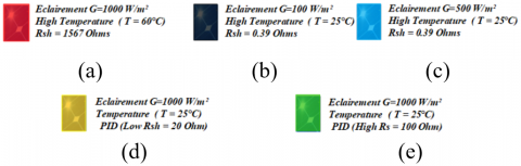
Figure 8 shows the various faults applied to the PV array to have the mismatch phenomenon.
Figure 8. Different phenomena can be found, (a) high temperature, (b) partial shading (100w/m²), (c) partial shading (500w/m²), (d) a decrease in the parallel resistance and (e) an increase in the series resistance
6.1 Simulation of 16 (4×4) PV modules under various mismatch conditions
6.1.1 Voltage mismatch issue simulation
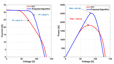
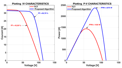
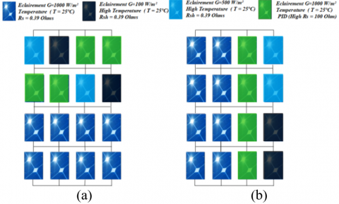
In Figure 9(a), the first test is carried out by creating the ageing scenario of 12.5% PV array, with the same number of PV modules under high temperature (60℃). The obtained arrangement by the proposed method is shown in Figure 9(b). The results of simulation are displayed in Figure 10, and Table 1. It shows a remarkable optimization of output power of about 20%. It is observed that FF is also increased by more than 39%. The proposed algorithm rearranges the modules realizing a PV module voltage balancing. The aim is to have, if possible, PV modules with the close voltage value on the same row. In this case 2, as shown in Figure 11(a), we apply a voltage mismatch on the PV array, by increasing the temperature (60℃) of 4 PV modules (25%), and also with the insertion of PV modules (25%) having a low parallel resistance value (ageing). The obtained arrangement by the proposed method is shown in Figure 11(b). As observed in Figure 12, and the Table 2, the proposed algorithm optimizes the output power by more than 30%, with a significant increase in the output voltage.
6.1.2 Current mismatch issue simulation
The second case of the simulation shows behaviour of the proposed algorithm under the different scenarios of current mismatch, such as partial shading and ageing of PV modules (Increase of series resistance).
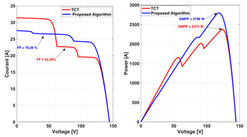
This case of simulation starts with a PV array having a quarter of PV modules under partial shading and high value of series resistance (ageing) as shown in Figure 13(a). Figure 13(b) shows the arrangement achieved using proposed method. The output power has been improved by minimizing losses. Figure 14, and Table 3 reveals an acceptable outcome, which results in a gain of about 12%. The proposed algorithm can reduce the effect of bypassing using the equalization of the rows currents.
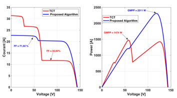
In the case 4, a PV array under 50% of infected PV modules is shown in Figure 15(a). The obtained arrangement by the proposed method is shown in Figure 15(b). After using the proposed algorithm, the maximum power has been improved by more than 24% as shown in Figure 16, and the Table 4. There is a substantial increase in output voltage due to elimination of the bypassed module problem (short-circuit mode).
6.1.3 Power mismatch simulation
In the last part of the simulation, the proposed algorithm is applied to a more complex PV system. It is about a PV array having PV modules that degrade both voltage and current.
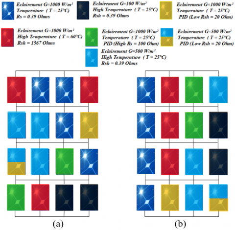
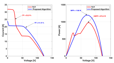
Figure 17(a) shows the last case studied in this part of a PV array having an important number of PV modules infected by different mismatch phenomena. The obtained arrangement by the proposed method is shown in Figure 17(b). As shown in Figure 18, and Table 5, the result obtained in this case is less than previous cases of power gain. Whereas, the shape of P-V curve obtained is optimal (smooth curve with the minimum number of infection points), due to disabling of bypass diodes. The optimization of I-V and P-V characteristic curve is very important to easily find the GMPP global power point.
Case 1: 2 PV modules M(1,1) and M(2,1) are aged (Low Rsh ), With High temperature in M(1,4) and M(4,3).
Figure 9. PV array under 25% of infected modules, (a) TCT configuration, (b) proposed algorithm arrangement
Table 1. Simulation results of case 1
|
Configuration |
Pm |
Vm |
Im |
Loss% |
FF% |
|
TCT |
1823 |
79.37 |
22.97 |
46.99 |
43.51 |
|
Proposed Algorithm |
2511 |
90.14 |
27.86 |
26.99 |
82.83 |
Figure 10. I-V and P-V characteristic curve for case 1
Case 2: 4 PV modules M(1,1), M(1,2), M(2.1) and M(2.2) are aged (Low Rsh ), With High temperature in M(3,1), M(3,4), M(4,2) and M(4,3).
Figure 11. PV array under 50% of infected modules, (a) TCT configuration, (b) proposed algorithm arrangement
Figure 12. I-V and P-V characteristic curve of case 2
Table 2. Simulation results of case 2
|
Configuration |
Pm |
Vm |
Im |
Loss% |
FF% |
|
TCT |
1435 |
55.39 |
25.9 |
59.29 |
43.59 |
|
Proposed Algorithm |
2375 |
81.77 |
29.04 |
30.97 |
65.79 |
Case 3: 2 PV modules M(1,1) and M(1,2) are aged (High Rs), With a partial shading in M(1,3) and M(1,4).
Figure 13. PV array under 25% of infected modules, (a) TCT configuration, (b) proposed algorithm arrangement
Figure 14. I-V and P-V characteristic curve for case 3
Table 3. Simulation results of case 3
|
Configuration |
Pm |
Vm |
Im |
Loss% |
FF% |
|
TCT |
2374 |
123.9 |
19.16 |
30.98 |
52.29 |
|
Proposed Algorithm |
2798 |
118.9 |
23.6 |
18.66 |
70.26 |
Case 4: PV modules M(1,3) , M(1,4),M(2.1) and M(2.2) are aged (High Rs ), With a partial shading in M(1,1), M(1,2), M(2,3) and M(2,4).
Figure 15. PV array under 50% of infected modules, (a) TCT configuration, (b) proposed algorithm arrangement
Table 4. Simulation results of case 4
|
Configuration |
Pm |
Vm |
Im |
Loss% |
FF% |
|
TCT |
1474 |
57.36 |
25.7 |
57.14 |
32.84 |
|
Proposed Algorithm |
2311 |
118.1 |
19.52 |
32.83 |
71.02 |
Figure 16. I-V and P-V characteristic curve for case 4
Case 5: PV modules M(2,1), M(2,2), M(3,1), M(3,2), M(4,3), and M(4,4) are Shaded, M(3.3), M(4,1) are aged (high Rs), Over temperature in M(1.1), M(1,4) and M(4.2), M(2,4) and M(3,1) are aged (Low Rsh).
Figure 17. PV array under 75% PV modules infected, (a) TCT configuration, (b) proposed algorithm arrangement
Figure 18. I-V and P-V characteristic curve for case 5
Table 5. Simulation results of case 5
|
Configuration |
Pm |
Vm |
Im |
Loss% |
FF% |
|
TCT |
975.2 |
76.56 |
12.74 |
71.65 |
25.21 |
|
Proposed Algorithm |
1196 |
71.92 |
16.64 |
65.22 |
41.15 |
6.2 Comparison with GA and SUDOKU methods
To further evaluate performance of the proposed algorithm, it is imperative to test their performance against meta-heuristic methods, such as genetic algorithm (GA) method. The obtained results are good compared to conventional methods. In the current work, we compare the proposed algorithm with GA and Su Do Ku methods. In the GA method, the author applies the evolutionary adaptive heuristic search nature of the genetic algorithm to find the optimal PV array configuration [23]. Therefore, the output power can be maximized by reducing the row current difference under every moment and every shading condition. Hence, a fine tuning of the three GA parameters is carried out as shown in Table 6.
Table 6. GA method parameters
|
Population size (567 bits/chromosome) |
10 |
|
Crossover |
1 |
|
Mutation |
0.02 |
|
Iterations |
100 |
An array of 81(9 × 9) PV modules connected in TCT configuration is exposed to three different shading schemes including (Short and wide shadow, and short and narrow shadow). In all three cases, the performance of PV array reconfigured by the proposed algorithm is compared to the initial configuration TCT, SuDoKu algorithm and GA.
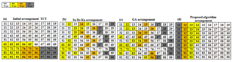
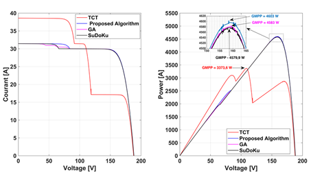
In the case of short and wide shadow, as shown in Figure 19 (a), a PV array connected in TCT is under four different levels of insolation. In the first group, the irradiation is 900 W/m². The second group gets 600 W/m². The third and fourth groups are irradiated with 400 W/m² and 200 W/m², respectively. Moreover, Figure 19(b), 19(c) and Figure 19(d) reveal the shade dispersion using SuDoKu arrangement, GA arrangement and proposed algorithm arrangement, respectively. It can be seen that the power increases with the proposed algorithm compared to the initial interconnection scheme TCT, SuDoKu method and the GA algorithm. As shown in Figure 20, the I-V and P-V curves clearly indicate that the proposed algorithm method maintains a relatively smooth curve with the minimum number of infection points (local PPM) and a high PPM voltage compared to the initial TCT interconnection scheme. Currents, voltages and power calculations are tabulated in Table 7, for TCT configuration, SuDoKu algorithms, GA and proposed algorithms, respectively.
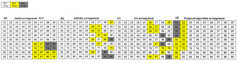
In the last case (short and narrow shadow), from Figure 21(a), a same PV array configuration under three irradiation levels, including 900 W/m²,600 W/m², and 400 W/m². Figure 21(b), Figure 21(c) and Figure 21(d) shown how the algorithms compared dispersed the shading, the proposed algorithm has superiority in output power. Furthermore, the proposed algorithm has very smooth I-V and P-V curves with reduced infection points, it was capable to minimize the difference between the induced currents in the rows, the results are shown in the Figure 22 and Table 8.
Another very important way of comparison, it is about the simplicity of the implementation, the proposed algorithm is robust and reliable, it is less complex to apply for a complex PV array in terms of calculations, coding and compilation.
6.3 Performance evaluation based on energy saving
Firstly, the author begins by the voltage mismatch that’s occur by the temperature variation, Potential Induced Degradation (PID) loss in solar cells and the other failures like diode failure, cells interconnect failure breakage. etc. those causses influence in the voltage output of the PV module. In the case 1 and 2, the PV system (4 × 4 size) is under poor conditions infect the output voltage by 12.5% and 25% respectively. The proposed approach improves the output power by more than 680 W (20 %) for the case 1, and 940 W (28%) for the case 2, resulting in a significant increase in output voltage which is beneficial to the operation of the solar inverter. In the second mismatch type that’s the current mismatch, the author carried out a simulation for two sizes of PV system, in the case 3 and 4, a PV array with 16 modules (4 × 4 size) interconnected in TCT is in poor conditions infects the output current as much as 25% and 50% respectively. The saved output power after applying the proposed algorithm is 424 W (12%) and 837 W (24%) for the two cases respectively. For cases 6 and 7, the current mismatch is also simulated in a larger PV array, which consists of 81 PV modules (size 9*9) interconnected in TCT. In the case of a short and wide shadow (case 6), the output power of the proposed approach is higher than that of the TCT, Sudoku and GA algorithms, with respectively 1229.6 W, 23.3 W and 19.9 W. Moreover, in the case 7 (short and narrow shadow), the proposed algorithm has a superiority in output power by 332.5 W, 56.8 W and 35.6 W compared by the TCT, SuDoKu and GA respectively. Finally, for the power mismatch, the proposed algorithm was evaluated in a PV array composed of 16 modules (4×4) under high degradation (75% modules PV affected by both the voltage and current mismatch), as a result, the proposed method contributed by 220 W with smoothed I-V and P-V curves. The findings above are summarized in the Table 9. As shown, the output power generated by the proposed technique is higher than that of the TCT, SuDoKu and GA methods for all seven cases. Moreover, the speed of the proposed algorithm helps to reach the optimal PV array architecture in the shortest time by rearranging the PV panels, which is a remarkable feature. Therefore, in the following section the author will present a comparative study of the calculation time of the examined algorithms.
6.4 Analysis based on computation timing
In order to validate the proposed algorithm, a comparison of the computation times is carried out. This is done under the same conditions on an Intel core i5 processor (2 cores of 2.4 GHz), and 6 GB of memory installed with a 64-bit Windows 7 operating system, the resultants are shown in the Table 10.
Note that the principle of the evolutionary methods such as GA is to generate a random initialization and to evolve optimal solutions after the operations of crossover, chromosome selection, and individual mutation. However, it is worth mentioning that the performance of the GA is influenced by the parameters of the algorithm; therefore, the corresponding operators of the GA method are carefully tuned by trial and error to achieve optimal performance. Therefore, in order to know the average speed of the studied algorithms, the minimum and maximum computation times are recorded for 10 different trails of the proposed and GA methods. According to the table, the proposed method clearly always arrives at the best solution compared to the GA method. Therefore, the GA method tends to converge into a local optimum. Hence, executing the code several times is necessary in order to get the global optimum. This involves more loss of computation time.
Figure 19. Shading pattern for case 6 (a) TCT interconnection scheme (b) shade dispersion with Su Do Ku arrangement, (c) shade dispersion with GA arrangement, and (d) shade dispersion with proposed arrangement
Figure 20. I-V and P-V characteristic curve for case 6
Figure 21. Shading pattern for case 7 (a) TCT interconnection scheme, (b)shade dispersion with Su Do Ku arrangement, (c)shade dispersion with GA arrangement, and (d) shade dispersion with Proposed arrangement
Figure 22. I-V and P-V characteristic curve for case 7
Table 7. Location of local and global PPM in TCT, SU DO KU, GA arrangement and proposed algorithm for case 6
|
Arrangement |
Row
Features |
Row1 |
Row2 |
Row3 |
Row4 |
Row5 |
Row6 |
Row7 |
Row8 |
Row9 |
|
TCT Arrangement |
$\sum{{{I}_{m}}}$ |
8.1 |
6.6 |
3.6 |
||||||
|
$\sum{{{V}_{m}}}$ |
5 |
6 |
9 |
|||||||
|
${{P}_{out}}$ |
40.5 |
39.6 |
32.4 |
|||||||
|
$PPM[W]$ |
Global PPM (3373.6) |
Local PPM1 |
Local PPM2 |
|||||||
|
Sudoku Arrangement |
$\sum{{{I}_{m}}}$ |
6.3 |
6.6 |
6.3 |
6.6 |
|||||
|
$\sum{{{V}_{m}}}$ |
9 |
4 |
9 |
4 |
||||||
|
${{P}_{out}}$ |
56.7 |
26.4 |
56.7 |
26.4 |
||||||
|
$PPM[W]$ |
Global PPM (4579.9) |
Local PPM1 |
Global PPM (4579.9) |
Local PPM1 |
||||||
|
GA Arrangement |
$\sum{{{I}_{m}}}$ |
6.6 |
6.3 |
6.4 |
6.6 |
6.3 |
6.5 |
6.3 |
6.6 |
|
|
$\sum{{{V}_{m}}}$ |
3 |
9 |
5 |
3 |
9 |
4 |
9 |
3 |
||
|
${{P}_{out}}$ |
19.8 |
56.7 |
32 |
19.8 |
56.7 |
26 |
56.7 |
19.8 |
||
|
$PPM[W]$ |
Local PPM1 |
Global PPM (4583.3) |
Local PPM3 |
Local PPM1 |
Global PPM (4583.3) |
Local PPM2 |
Global PPM (4583.3) |
Local PPM1 |
||
|
Proposed Algorithm Arrangement |
$\sum{{{I}_{m}}}$ |
6.3 |
6.6 |
|||||||
|
$\sum{{{V}_{m}}}$ |
9 |
4 |
||||||||
|
${{P}_{out}}$ |
56.7 |
26.4 |
||||||||
|
$PPM[W]$ |
Global PPM (4603.2) |
Local PPM1 |
||||||||
Table 8. Location of local and global PPM in TCT, SU DO KU, GA arrangement and proposed algorithm for Case 7
|
Arrangement |
Row
Features |
R1 |
R2 |
R3 |
R4 |
R5 |
R6 |
R7 |
R8 |
R9 |
|
|
TCT Arrangement |
$\sum{{{I}_{m}}}$ |
8.1 |
7.4 |
6.9 |
|||||||
|
$\sum{{{V}_{m}}}$ |
5 |
7 |
9 |
||||||||
|
${{P}_{out}}$ |
40.5 |
51.8 |
62.1 |
||||||||
|
$PPM[W]$ |
Local PPM1 |
Local PPM2 |
Global PPM (4998.3) |
||||||||
|
Sudoku Arrangement |
$\sum{{{I}_{m}}}$ |
7.8 |
7.5 |
6.8 |
7.8 |
7.3 |
7.1 |
||||
|
$\sum{{{V}_{m}}}$ |
3 |
6 |
9 |
3 |
7 |
8 |
|||||
|
${{P}_{out}}$ |
23.4 |
45 |
61.2 |
23.4 |
51.1 |
56.8 |
|||||
|
$PPM[W]$ |
Local PPM1 |
Local PPM2 |
Global PPM (5274) |
Local PPM1 |
Local PPM3 |
Local PPM4 |
|||||
|
GA Arrangement |
$\sum{{{I}_{m}}}$ |
7.5 |
7.6 |
7.3 |
7.5 |
7.3 |
7 |
||||
|
$\sum{{{V}_{m}}}$ |
6 |
2 |
8 |
6 |
8 |
9 |
|||||
|
${{P}_{out}}$ |
45 |
15.2 |
58.4 |
45 |
58.4 |
63 |
|||||
|
$PPM[W]$ |
Local PPM2 |
Local PPM1 |
Local PPM3 |
Local PPM2 |
Local PPM3 |
Global PPM( 5295.2) |
|||||
|
Proposed Algorithm Arrangement |
$\sum{{{I}_{m}}}$ |
7.3 |
7.5 |
7.8 |
|||||||
|
$\sum{{{V}_{m}}}$ |
9 |
5 |
2 |
||||||||
|
${{P}_{out}}$ |
65.7 |
37.5 |
15.6 |
||||||||
|
$PPM[W]$ |
Global PPM (5330.8) |
Local PPM2 |
Local PPM1 |
||||||||
Table 9. Power output summary for TCT, SuDoKu, GA and the proposed approach for different array sizes
|
Array size |
Mismatch type |
Method |
Maximum power (W) |
Power enhancement using proposed method (W) |
|
|
4 × 4 modules |
Voltage mismatch |
Case 1 |
TCT |
1823 |
688 |
|
Proposed Algorithm |
2511 |
||||
|
Case 2 |
TCT |
1435 |
940 |
||
|
Proposed Algorithm |
2375 |
||||
|
Current mismatch |
Case 3 |
TCT |
2374 |
424 |
|
|
Proposed Algorithm |
2798 |
||||
|
Case 4 |
TCT |
1474 |
837 |
||
|
Proposed Algorithm |
2311 |
||||
|
Power mismatch |
Case 5 |
TCT |
975.2 |
220.8
|
|
|
Proposed Algorithm |
1196 |
||||
|
9 × 9 modules |
Current mismatch |
Case 6 |
TCT |
3373.6 |
1229.6 vs TCT 23.3 vs SuDoKu 19.9 vs GA |
|
SuDoKu |
4579.9 |
||||
|
GA |
4583.3 |
||||
|
Proposed algorithm |
4603.2 |
||||
|
Case 7 |
TCT |
4998 .3 |
332.5 vs TCT 56.8 vs SuDoKu 35.6 vs GA |
||
|
SuDoKu |
5274 |
||||
|
GA |
5295.2 |
||||
|
Proposed algorithm |
5330.8 |
||||
Table 10. Minimum, maximum and average computational time for different case using GA, and proposed algorithms
|
Case |
Method |
Min computational time (s) |
Max computational time (s) |
Average computational time (s) |
|
Case 6 |
GA |
40.967 |
54.548 |
46.0828 |
|
Proposed algorithm |
0.323 |
0.414 |
0.3728 |
|
|
Case 7 |
GA |
39.682 |
56.129 |
45.018 |
|
Proposed algorithm |
0.327 |
0.592 |
0.402. |
In this study, a new optimization algorithm for solar PV systems is employed to achieve the maximum power production under any mismatch effects. The general idea of the proposed method is based on the relocation of the installed PV modules in order to balance their physical values (current, voltage and power) as follows:
In brief, we want to electrically balance the PV system to avoid:
A software validation has been done using MATLAB/Simulink. The proposed approach provides good results. However, A comparative study was done with the SuDoKu and GA algorithms. The results obtained show the superiority of the proposed algorithm in:
The proposed method is robust and reliable, simple to apply for a large PV array and easy to code and compile.
The authors gratefully acknowledge the Algerian General Direction of Research (DGRSDT) for providing the facilities and the financial funding of this project.
|
BL |
bridge link |
|
CS |
competence square |
|
IEA |
International Energy Agency |
|
GA |
genetic algorithm |
|
GMPP |
global maximum power point |
|
HC |
honey-comb |
|
HC |
honey comb |
|
PV |
photovoltaic |
|
MPPT |
Maximum power point tracking |
|
MPP |
Maximum power point |
|
SP |
series parallel |
|
TCT |
total cross tied |
|
STC |
Standard test condition |
|
Rsh |
Shunt resistance |
|
Rs |
Series resistance |
|
FF |
Fill factor |
|
PID |
Potential Induced Degradation |
[1] International Energy Agency and I. E. Agency, World Energy Outlook 2011. OECD, 2011.
[2] Compaan, A.D. (2006). Photovoltaics: Clean power for the 21st century. Solar Energy Materials and Solar Cells, 90(15): 2170-2180. https://doi.org/10.1016/j.solmat.2006.02.017
[3] Amponsah, N.Y., Troldborg, M., Kington, B., Aalders, I., Hough, R.L. (2014). Greenhouse gas emissions from renewable energy sources: A review of lifecycle considerations. Renewable and Sustainable Energy Reviews, 39: 461-475. https://doi.org/10.1016/j.rser.2014.07.087
[4] Bevan, G. (2012). Renewable energy and climate change. Significance, 9(6): 8-12. https://doi.org/10.1111/j.1740-9713.2012.00614.x
[5] IEA. (2019). ‘World Energy Outlook 2019’, IEA, Paris. https://www.iea.org/reports/world-energy-outlook-2019.
[6] Stetz, T., Marten, F., Braun, M. (2012). Improved low voltage grid-integration of photovoltaic systems in Germany. IEEE Transactions on Sustainable Energy, 4(2): 534-542. https://doi.org/10.1109/TSTE.2012.2198925
[7] Celik, A.N. (2002). Optimisation and techno-economic analysis of autonomous photovoltaic–wind hybrid energy systems in comparison to single photovoltaic and wind systems. Energy Conversion and Management, 43(18): 2453-2468. https://doi.org/10.1016/S0196-8904(01)00198-4
[8] Al Garni, H., Kassem, A., Awasthi, A., Komljenovic, D., Al-Haddad, K. (2016). A multicriteria decision making approach for evaluating renewable power generation sources in Saudi Arabia. Sustainable Energy Technologies and Assessments, 16: 137-150. https://doi.org/10.1016/j.seta.2016.05.006
[9] Huang, B.J., Lin, T.H., Hung, W.C., Sun, F.S. (2001). Performance evaluation of solar photovoltaic/thermal systems. Solar Energy, 70(5): 443-448. https://doi.org/10.1016/S0038-092X(00)00153-5
[10] Chamberlin, C.E., Lehman, P., Zoellick, J., Pauletto, G. (1995). Effects of mismatch losses in photovoltaic arrays. Solar Energy, 54(3): 165-171. https://doi.org/10.1016/0038-092X(94)00120-3
[11] El-Dein, M.S., Kazerani, M., Salama, M.M.A. (2012). An optimal total cross tied interconnection for reducing mismatch losses in photovoltaic arrays. IEEE Transactions on Sustainable Energy, 4(1): 99-107. https://doi.org/10.1109/TSTE.2012.2202325
[12] Kavlak, G., McNerney, J., Trancik, J.E. (2018). Evaluating the causes of cost reduction in photovoltaic modules. Energy Policy, 123: 700-710. https://doi.org/10.1016/j.enpol.2018.08.015
[13] Hirst, L.C., Ekins-Daukes, N.J. (2011). Fundamental losses in solar cells. Progress in Photovoltaics: Research and Applications, 19(3): 286-293. https://doi.org/10.1002/pip.1024
[14] Singh, P., Ravindra, N.M. (2012). Temperature dependence of solar cell performance-An analysis. Solar Energy Materials and Solar Cells, 101: 36-45. https://doi.org/10.1016/j.solmat.2012.02.019
[15] Skoplaki, E., Palyvos, J.A. (2009). On the temperature dependence of photovoltaic module electrical performance: A review of efficiency/power correlations. Solar Energy, 83(5): 614-624. https://doi.org/10.1016/j.solener.2008.10.008
[16] Sharma, V., Chandel, S.S. (2013). Performance and degradation analysis for long term reliability of solar photovoltaic systems: A review. Renewable and Sustainable Energy Reviews, 27: 753-767. https://doi.org/10.1016/j.rser.2013.07.046
[17] Köntges, M., Kunze, I., Kajari-Schröder, S., Breitenmoser, X., Bjørneklett, B. (2010). Quantifying the risk of power loss in PV modules due to micro cracks. In 25th European Photovoltaic Solar Energy Conference, Valencia, Spain, pp. 3745-3752.
[18] Da Luz, C.M.A., dos Santos Vicente, P., Tofoli, F.L., Vicente, E.M. (2016). Influence of series and shunt resistances in the ideality factor of photovoltaic modules. In 2016 12th IEEE International Conference on Industry Applications (INDUSCON), pp. 1-6. https://doi.org/10.1109/INDUSCON.2016.7874588
[19] Rao, P.S., Ilango, G.S., Nagamani, C. (2014). Maximum power from PV arrays using a fixed configuration under different shading conditions. IEEE Journal of Photovoltaics, 4(2): 679-686. https://doi.org/10.1109/JPHOTOV.2014.2300239
[20] Ramabadran, R., Mathur, B. (2009). Matlab based modelling and performance study of series connected SPVA under partial shaded conditions. Journal of Sustainable Development, 2(3): 85-94. https://doi.org/10.5539/jsd.v2n3p85
[21] Buddha, S.T. (2011). Topology reconfiguration to improve the photovoltaic (PV) array performance. Arizona State University, 11(1): 147-173.
[22] Rani, B.I., Ilango, G.S., Nagamani, C. (2013). Enhanced power generation from PV array under partial shading conditions by shade dispersion using Su Do Ku configuration. IEEE Transactions on Sustainable Energy, 4(3): 594-601. https://doi.org/10.1109/TSTE.2012.2230033
[23] Deshkar, S.N., Dhale, S.B., Mukherjee, J.S., Babu, T.S., Rajasekar, N. (2015). Solar PV array reconfiguration under partial shading conditions for maximum power extraction using genetic algorithm. Renewable and Sustainable Energy Reviews, 43: 102-110. https://doi.org/10.1016/j.rser.2014.10.098
[24] Babu, T.S., Ram, J.P., Dragičević, T., Miyatake, M., Blaabjerg, F., Rajasekar, N. (2017). Particle swarm optimization based solar PV array reconfiguration of the maximum power extraction under partial shading conditions. IEEE Transactions on Sustainable Energy, 9(1): 74-85. https://doi.org/10.1109/TSTE.2017.2714905
[25] Abete, A., Barbisio, E., Cane, F., Demartini, P. (1990). Analysis of photovoltaic modules with protection diodes in presence of mismatching. In IEEE Conference on Photovoltaic Specialists, 1005-1010. https://doi.org/10.1109/PVSC.1990.111769
[26] Luque, A., Hegedus, S. (Eds.). (2011). Handbook of Photovoltaic Science and Engineering. John Wiley & Sons.
[27] Wenham, S.R., Green, M.A., Watt, M.E., Corkish, R., Sproul, A. (2013). Applied photovoltaics. Routledge.
[28] Shirzadi, S., Hizam, H., Wahab, N.I.A. (2014). Mismatch losses minimization in photovoltaic arrays by arranging modules applying a genetic algorithm. Solar Energy, 108: 467-478. https://doi.org/10.1016/j.solener.2014.08.005