Aziz El Janati El Idrissi* | Mohsin Beniysa | Adel Bouajaj | Mohammed Réda Britel
© 2021 IIETA. This article is published by IIETA and is licensed under the CC BY 4.0 license (http://creativecommons.org/licenses/by/4.0/).
OPEN ACCESS
In this paper, stable and adaptive neural network compensators are proposed to control the uncertain permanent magnet synchronous motor (PMSM). Firstly, the overall uncertainties caused by mathematical modelling, parameters variation during operation and external load torque disturbances are modelled. Secondly, a new motion control scheme, where (d-q) current loops are dotted by two on-line tuning neural network compensators (NNCs), is used to compensate these uncertainties. As a result, the speed control loop is processed easily by proportional integral (PI) controller. Stability of the closed-loop system is also designed according to the Lyapunov stability. Compared to classical vector control, the simulations of PMSM system at different speeds including nominal, low and high speed, with and without uncertainties, show the effectiveness of the proposed control scheme.
uncertain PMSM, adaptive neural network, compensator, parameter uncertainties, Lyapunov stability
In the past two decades, many problems of uncertain nonlinear systems such as PMSM, manipulators, robots etc. are intensively studied in the automatic research field. PMSM is increasingly used in industrial applications due to its high efficiency, high speed, high power density, low cost and large torque to inertia ratio [1, 2]. But it is still a challenging domain of research to control these types of motors perfectly, because of their mathematical modelling, multi-variability, nonlinearities, parameters uncertainties, high degrees of freedom and external disturbances. These problems can cause undesired behavior of PMSM that can extremely destroy the stabilization of the motor drive. However, traditional control techniques cannot be used in this case [3]. In order to overcome these drawbacks, many adaptive techniques are proposed in recent years. The most popular of them are backstepping control with disturbance observer [4], unknown disturbance estimation with a hybrid sliding mode observer [5], and adaptive sliding model control [6, 7]. However, these mentioned control methods require the exact mathematical model of the dynamical system, but the model is approximated by ignoring some physical phenomena. To overcome this problem others modern optimized and intelligent techniques are proposed in the literatures [8-12].
In recent years, neural networks (NN) have always been considered as an efficient method in control of linear and nonlinear systems, due to its high accuracy and robustness against internal and external disturbances [13-16]. The NN is a set of the neuron’s structures using training algorithm to adjust the NN weight’s [17]. The online weight updating mechanism is an extended version of training algorithm with a simple structure by adding an adaptive term to guarantee the robustness of uncertainty. Extended version of neural networks control has been found one of the most popular and conventional tools in engineering control, identification and functional approximations [18-20].
The NN control has strong ability of handling uncertain information and can be easily used in the engineering control systems that are too complex to have an exact mathematical model. Actually, NN techniques have been developed in both continuous and discrete-time, but the techniques implemented in discrete-time have the favor that they can be directly implemented in digital hardware [21-32]. Unfortunately, one of the most important problems of NN control system analysis is the stability, and especially when the system is in discrete-time [21, 22]. Over the past decade, the stability and stabilization of NN systems have been considered as an essential and necessary area of researches [21-27]. However, stability analysis of NN systems was studied mainly by Lyapunov stability theory and others different kinds of its extended versions [28-32].
The main objective of this work is to use an intelligent dynamic approach based on two on-line tuning neural networks compensators (NNCs), which can adapt their weights dynamically to any uncertainty in the PMSM drives. This adaptation allows the NNCs to eliminate all disturbances related to nonlinearities uncertainties caused by mathematical modelling, external disturbance affected by the external load and parameters uncertainty. The discrete Lyapunov function is also considered to verify the stability of the PMSM under these uncertainties. In order to validate the effectiveness of the proposed approach we used several inputs references data for respective simulation tests. The simulation results are discussed and compared to those obtained in classical vector control. The results indicate that the proposed approach is successful and simple to control PMSM systems in spite of the uncertainty problems.
By considering the simplifying conditions, assumptions and physical laws, the three-phase mathematical model of PMSM can be expressed easily in three-phase (abc) frame [5-17]. Then, by developing this coupled three-phase mathematical model of PMSM, the (dq) axis of current, voltage and flux can be also obtained from Park and Concordia transformations [33]. So, according to the above steps the electromechanical behavior of PMSM system can be described by the following first order differential equations [33]:
$\left\{\begin{array}{l}L_{d} \frac{d i_{d}}{d t}=u_{d}-R i_{d}+p L_{q} \omega_{r} i_{q} \\ L_{q} \frac{d i_{q}}{d t}=u_{q}-R i_{q}-p L_{d} \omega_{r} i_{d}-p \varphi_{v} \omega_{r} \\ J \frac{d \omega_{r}}{d t}=T_{e}-T_{r}-B \omega_{r} \\ \frac{d \theta_{r}}{d t}=\omega_{r} \\ \omega_{e}=p \omega_{r} \\ T_{e}=1.5 p\left(\varphi_{v} i_{q}+\left(L_{d}-L_{q}\right) i_{d} i_{q}\right)\end{array}\right.$ (1)
where, R represents the stator resistance, $\theta_{r}$ represents the rotor position, ud and uq represent the stator voltages at rotational reference frame, id and iq represent the direct and quadrature stator currents, $\omega_{r}$ and $\omega_{e}$ represent the electrical and mechanical rotor speeds, $\varphi_{v}$ represents the stator flux linkage due to the permanent magnet, Te represents the electrical torque, p represents the number of pole pairs, J represents the rotor inertia, B represents the friction, Ld and Lq represent the direct and quadrature stator inductances and Tr represents the mechanical load torque.
Furthermore, by using the following notations: $i_{d}(k)=x_{1}(k), i_{d}(k+1)=x_{2}(k), \quad i_{q}(k)=x_{3}(k)$, $i_{q}(k+1)=x_{4}(k), \omega_{r}(k)=x_{5}(k), \omega_{r}(k+1)=x_{6}(k)$, $\theta_{r}(k)=x_{7}(k), \theta_{r}(k+1)=x_{8}(k), T_{e}(k)=x_{9}(k), T_{e}(k+$ $1)=x_{10}(k)$ the dynamic of the PMSM can be rewritten in the Brunovsky discrete-time domain form by the following system of equations, according to Newton discretization method:
$\left\{\begin{array}{l}x_{1}(k+1)=x_{2}(k) \\ x_{2}(k+1)=x_{2}(k)+\left(u_{d}(k)-R x_{2}(k)+p L_{q} x_{4}(k) x_{6}(k)\right)\left(\frac{T_{s}}{L_{d}}\right) \\ x_{3}(k+1)=x_{4}(k) \\ x_{4}(k+1)=x_{4}(k)+\left(u_{d}(k)-R x_{4}(k)-p L_{q} x_{2}(k) x_{6}(k)-p \varphi_{v} x_{6}(k)\right)\left(\frac{T_{s}}{L_{d}}\right) \\ x_{5}(k+1)=x_{6}(k) \\ x_{6}(k+1)=x_{6}(k)+\left(x_{10}(k)-T_{r}-B x_{6}(k)\right)\left(\frac{T_{s}}{J}\right) \\ x_{7}(k+1)=x_{8}(k) \\ x_{8}(k+1)=x_{8}(k)+x_{6}(k) T_{s} \\ x_{9}(k+1)=x_{10}(k) \\ x_{10}(k+1)=1.5 \mathrm{p}\left(\varphi_{v} x_{4}(k+1)+\left(L_{d}-L_{q}\right) x_{2}(k+1) x_{4}(k+1)\right)\end{array}\right.$ (2)
where, Ts is the sampling time. In the fact, the parameters $\varphi_{v}, R, L_{d}, L_{q}, B, J$, and load torque $T_{r}$ are uncertain during the operation, then:
$\begin{array}{lll}\hat{L}_{d}=L_{d}+\tilde{L}_{d} & \hat{J}=J+\tilde{J} & \widehat{T}_{r}=T_{r}+\widetilde{T}_{r} \\ \hat{L}_{q}=L_{q}+\tilde{L}_{q} & \hat{R}=R+\widetilde{R} & \hat{\varphi}_{v}=\varphi_{v}+\tilde{\varphi}_{v} \\ \hat{B}=B+\widetilde{B} & \end{array}$ (3)
where, the parameters defined by cap depict the parameter actual values, the tiled parameters depict the individual errors and the parameters without accent depict constant (nominal) values. Substituting nominal parameters in Eq. (2) by those caped in Eq. (3), the uncertain PMSM can be modelled by the following equations:
$\left\{\begin{array}{l}x_{1}(k+1)=x_{2}(k) \\ x_{2}(k+1)=x_{2}(k)+\left(u_{d}(k)-R x_{2}(k)+p L_{q} x_{4}(k) x_{6}(k)\right)\left(\frac{T_{s}}{L_{d}}\right) \\ \left(-\tilde{R} x_{2}(k)+p L_{q} x_{4}(k) x_{6}(k)- \left(u_{d}(k)-R x_{2}(k)+p L_{q} x_{4}(k) x_{6}(k)\right)\left(\frac{L_{d}}{L_{d}}\right)\right)\left(\frac{T_{s}}{L_{d}+\mathcal{L}_{d}}\right)=f_{d}(x(k))+\tau_{d}(k)+d_{d}(k) \\ x_{3}(k+1)=x_{4}(k) \\ x_{4}(k+1)=x_{4}(k)+\left(u_{d}(k)-R x_{4}(k)-p L_{q} x_{2}(k) x_{6}(k)-p \varphi_{v} x_{6}(k)\right)\left(\frac{T_{s}}{L_{d}}\right) \\+\left(-R x_{4}(k)-p L_{d} x_{2}(k) x_{6}(k)-p \varphi_{v} x_{6}(k)- \left(u_{q}(k)-R x_{4}(k)-p L_{d} x_{2}(k) x_{6}(k)-p \varphi_{v} x_{6}(k)\right)\left(\frac{L_{q}}{L_{q}}\right)\right)\left(\frac{T_{s}}{L_{q}+L_{q}}\right)=f_{q}(x(k))+\tau_{q}(k)+d_{q}(k) \\ x_{5}(k+1)=x_{6}(k) \\ x_{6}(k+1)=x_{6}(k)+\left(x_{10}(k)-T_{r}-B x_{6}(k)\right)\left(\frac{T_{s}}{J}\right) \\+\left(-\tilde{T}_{r}-\tilde{B} x_{6}(k)-\left(x_{10}(k)-T_{r}-B x_{6}(k)\right)\left(\frac{\tilde{J}}{J}\right)\right)\left(\frac{T_{s}}{J+\tilde{J}}\right)=x_{6}(k)+\left(x_{10}(k)-T_{r}-Bx_{6}(k)\right)\left(\frac{T_{s}}{J}\right)+d_{\omega}(k) \\ x_{7}(k+1)=x_{8}(k) \\ x_{8}(k+1)=x_{8}(k)+x_{6}(k) T_{s} \\ x_{9}(k+1)=x_{10}(k) \\ x_{10}(k+1)=1.5 \mathrm{p}\left(\varphi_{v} x_{4}(k+1)+\left(L_{d}-L_{q}\right) x_{2}(k+1) x_{4}(k+1)\right) \\+1.5 \mathrm{p}\left(\tilde{\varphi}_{v} x_{4}(k+1)+\left(\tilde{L}_{d}-\tilde{L}_{q}\right) x_{2}(k+1) x_{4}(k+1)\right) 1.5 \mathrm{p}\left(\varphi_{v} x_{4}(k+1)+\left(L_{d}-L_{q}\right) x_{2}(k+1) x_{4}(k+1)\right)+d_{T}(k) \end{array}\right.$ (4)
where, $x_{i}(k) \in \mathbb{R}^{10}, i=\{1,2 \ldots, 10\}$, and $\tau_{i}(k) \in \mathbb{R}^{2}, i=\{\mathrm{d}, \mathrm{q}\}$, The vector $d_{i}(k) \in \mathbb{R}^{4}, i=\{\mathrm{d}, \mathrm{q}, \omega, \mathrm{T}\}$ denotes an unknown disturbance acting on the system at the kth time with known constant.
From the Eq. (4) we conclude that the output $\tau_{i}(k)$ is related to the uncertain control input $u_{i}(k), i=\{d, q\}$ through the following nonlinear expression:
$\left\{\begin{array}{l}\tau_{d}(k)=u_{d}(k)\left(\frac{T_{s}}{L_{d}}\right)+\left(\begin{array}{c}-\tilde{R} x_{2}(k)+p \tilde{L}_{q} x_{4}(k) x_{6}(k)- \\ \left(u_{d}(k)-R x_{2}(k)+p L_{q} x_{4}(k) x_{6}(k)\right)\left(\frac{\tilde{L}_{d}}{L_{d}}\right)\end{array}\right)\left(\frac{T_{s}}{L_{d}+\tilde{L}_{d}}\right) \\ \tau_{q}(k)=u_{q}(k)\left(\frac{T_{s}}{L_{q}}\right)+\left(\begin{array}{c}-\tilde{R} x_{4}(k)-p \tilde{L}_{d} x_{2}(k) x_{6}(k)-p \tilde{\varphi}_{v} x_{6}(k)- \\ \left(u_{q}(k)-R x_{4}(k)-p L_{d} x_{2}(k) x_{6}(k)-p \varphi_{v} x_{6}(k)\right)\left(\frac{\tilde{L}_{q}}{L_{q}}\right)\end{array}\right)\left(\frac{T_{s}}{L_{q}+\tilde{L}_{q}}\right)\end{array}\right.$ (5)
Since a backlash is a dynamic nonlinearity, the uncertainties in Eq. (5) can be modelled by the following backlash in discrete time domain [21, 22]:
$\begin{aligned} \tau_{i}(k) &=\operatorname{Backlash}\left(\tau_{i}(k-1), u_{i}(k-1), u_{i}(k)\right) \\ &=\left\{\begin{array}{cc}m_{i} u_{i}(k) & \text { if }\left(\left(u_{i}(k)>0\right) \text { and } u_{i}(k-1)=m_{i}\left(\tau_{i}(k-1)-d_{i+}\right)\right) \\ & \text { if }\left(\left(u_{i}(k)<0\right) \text { and } u_{i}(k-1)=m_{i}\left(\tau_{i}(k-1)-d_{i-}\right)\right)\\ \text { 0 } & \text { Otherwise } \end{array}\right.\end{aligned}$ (6)
where, $u_{i}(k-1)$ and $u_{i}(k)$ are the inputs of backlash function, $\tau_{i}(k-1)$ is the state, and $m_{i}, d_{i+}$ and $d_{i-}$ are unknown values, $i=\{d, q\}$.
The control law of this nonlinear discrete-time control of PMSM system is based on the following assumptions [21, 22]:
Assumption 1: The desired trajectory is assumed to be bounded in the sense that $\left\|x_{(i, 1)}^{*}(k)\right\|^{T} \leq X_{(i, 1)}$ and $\left\|x_{(i, 2)}^{*}(k)\right\|^{T} \leq X_{(i, 2)}$ for a known bound $X_{(i, 1)}$ and $X_{(i, 2)}$, where $x_{(i, 1)}^{*}(k)$ is the delayed value of $x_{(i, 2)}^{*}(k), i=\{d, q\}$.
Assumption 2: The nonlinear function $f_{i}(x(k))$ is assumed to be unknown, but a fixed estimate $\hat{f}_{i}(x(k))$ is assumed known such that the functional estimation error $\tilde{\varepsilon}_{i}(x(k))=\hat{f}_{i}(x(k))-f_{i}(x(k))$ satisfies $\|\tilde{\varepsilon}(x(k))\| \leq$ $f_{i M}(x(k))$ for some known bounding function $f_{i M}(x(k)), i=$ $\{d, q\}$.
Assumption 3: The unknown disturbance is also assumed to satisfy: $\left\|\tau_{i}\right\| \leq \tau_{i M}$, with $\tau_{i M}(k)$ are a known positive constants, $i=\{d, q\}$.
Assumption 4: The unknown values $m_{i}, d_{i+}$ and $d_{i-}$ are bounded by known constants $M_{i}, D_{i+}$ and $D_{i-}$ as: $\left\|m_{i}\right\| \leq M_{i},\left\|d_{i+}\right\| \leq D_{i+}$ and $\left\|d_{i}\right\| \leq D_{i-}$.
Assumption 5: The dynamics of the backlash compensator is invertible. Its dynamic inverse is indicated by the following equation:
$u_{i}(k)=\operatorname{Backlash}^{-1}\left(u_{i}(k-1), w_{i}(k-1), w_{i}(k)\right)$ (7)
where, $w_{i}(k-1)$ and $w_{i}(k)$ are the signals input of the backlash inverse that generates the signal $u_{i}(k)$, which is subsequently sent into the backlash to generate $\tau_{i}(k)$.
Assumption 6: The parameters $m_{i}, d_{i+}$ and $d_{i-}$ used in the backlash inverse are exactly corrects.
Our objective is to control the speed and currents of uncertain PMSM such that the tracking errors of $x_{i}(k), i=\{1,2, \ldots, 10\}$ closely converge to zero in the presence of any uncertainty. To achieve this objective, the stable discrete-time adaptive neural networks compensators are used. To prove the stability of the system the Lyapunov function is applied.
3.1 Main scheme of the proposed technique
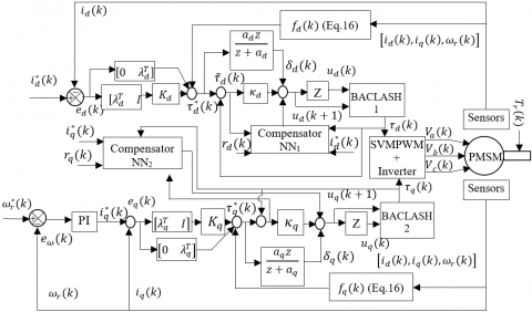
The tracking control system is presented schematically in Figure 1. The overall system consists of the uncertain PMSM coupled to variable external load disturbance, space vector pulse width modulation (SVPWM), voltage-source inverter (VSI), two backlash models, two estimated functions, two filters, two proportional-plus-derivative (PD) controllers, two NNCs and three essential loops.
Figure 1. Stable and adaptive scheme for uncertain PMSM control
The controllers employ a structure of cascade control loop including a speed loop and two inner current loops. Here, the controllers, which are used to stabilize the (dq)-axis currents error, are adopted according to $\lambda_{i}$ Hurwitz gains, which are followed by two inner PD controllers with gains $\left(K_{i}\right.$ and $\left.\kappa_{i}, i=\{d, q\}\right)$. The PI controller is also used to track the desired speed. As it can be seen from Figure 1, the electrical angular speed $\omega_{r}$ can be obtained from the position sensor, The currents $i_{d}$ and $i_{q}$ can be calculated from measured three-phase currents $i_{a}$ and $i_{b}$ by Park transformations.
According to the actual value of the angle $\theta_{r}$, the backlash outputs can be transformed, from the rotating (d, q) frame to the stator-fixed coordinates $(\alpha, \beta)$, to be the inputs of SVPWM that activates the transistors state of the inverter. Finally, the suitable stator voltages are applied on the motor with respect to the amplitude and the desired frequency. The uncertainty of PMSM destroys the tracking, and then the classical PD controllers are not capable to compensate it. To correct the errors due to this uncertainty, neural network compensators are used.
More details about the design procedure for the proposed control strategy (Figure 1) are presented step-by-step in the following subsection.
3.2 Discrete-time PI controller of the speed
To handle speed trajectory a PI controller is considered. The expressions of the proportional and integral controller gain respectively $K_{P}$ and $K_{I}$ are determined by the following equations [20]:
$\left\{\begin{array}{l}K_{I}=\frac{4 J R^{2}}{L_{q}^{2}} \\ K_{P}=\frac{K_{I} L_{q}}{R}\end{array}\right.$ (8)
This controller compares, at each iteration, the actual speed value with the desired speed value. Then, it processes the speed errors defined by the Eq. (9) by the Eq. (10) to track the desired speed perfectly.
$\left\{\begin{array}{l}e_{i}(k)=x_{i}^{*}(k)-x_{i}(k) \\ e_{i}(k+1)=x_{i}^{*}(k+1)-x_{i}(k+1) ; \quad i=\{5,6\}\end{array}\right.$ (9)
where, $e_{i}(k)$ and $e_{i}(k+1)$, represent the speed errors at discrete-times k and (k+1).
$\left\{\begin{array}{l}x_{9}^{*}(k)=x_{9}^{*}(k-1)+K_{P} e_{5}(k)+\left(K_{I} T_{s}-K_{P}\right) e_{5}(k-1) \\ x_{10}^{*}(k)=x_{10}^{*}(k-1)+K_{P} e_{6}(k)+\left(K_{I} T_{s}-K_{P}\right) e_{6}(k-1) \\ x_{9}^{*}(k+1)=x_{9}^{*}(k)+K_{P} e_{5}(k+1)+\left(K_{I} T_{s}-K_{P}\right) e_{5}(k) \\ x_{10}^{*}(k+1)=x_{10}^{*}(k)+K_{P} e_{6}(k+1)+\left(K_{I} T_{s}-K_{P}\right) e_{6}(k)\end{array}\right.$ (10)
For $i_{d}^{*}=0$ strategy, the desired trajectory of iq is related to the desired trajectory of the torque with the following equations:
$\left\{\begin{array}{l}x_{3}^{*}(k)=\frac{2}{3 p \varphi_{v}} x_{9}^{*}(k) \\ x_{3}^{*}(k+1)=\frac{2}{3 p \varphi_{v}} x_{9}^{*}(k+1) \\ x_{4}^{*}(k)=\frac{2}{3 p \varphi_{v}} x_{10}^{*}(k) \\ x_{4}^{*}(k+1)=\frac{2}{3 p \varphi_{1}} x_{10}^{*}(k+1)\end{array}\right.$ (11)
Hence, by substituting Eq. (10) in Eq. (11), the desired trajectory $i_{q}^{*}$ is related to the tracking errors of the speed with the following equations:
$\left\{\begin{array}{l}x_{3}^{*}(k)=x_{3}^{*}(k-1)+\frac{2}{3 p \varphi_{v}}\left(K_{p} e_{5}(k)+\left(K_{I} T_{s}-K_{p}\right) e_{5}(k-1)\right) \\ x_{3}^{*}(k+1)=x_{3}^{*}(k)+\frac{2}{3 p \varphi_{v}}\left(K_{p} e_{5}(k+1)+\left(K_{I} T_{s}-K_{p}\right) e_{5}(k)\right) \\ x_{4}^{*}(k)=x_{4}^{*}(k-1)+\frac{2}{3 p \varphi_{v}}\left(K_{p} e_{6}(k)+\left(K_{I} T_{s}-K_{p}\right) e_{6}(k-1)\right) \\ x_{4}^{*}(k+1)=x_{4}^{*}(k)+\frac{2}{3 p \varphi_{k}}\left(K_{p} e_{6}(k+1)+\left(K_{I} T_{s}-K_{p}\right) e_{6}(k)\right)\end{array}\right.$ (12)
3.3 Discrete-time adaptive neural networks compensators
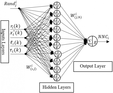
Figure 2. The structure of neural network compensators
The multi-layer perceptron neural networks (MLPNNs), used as compensators in this work (Figure 2), have dynamic weights between hidden and output neurons and static weights between input and hidden layers neurons. Consequently, they possess lesser number of weights to be updated and can be trained quickly and easily.
The concept of the adaptation technique law is to track precisely the desired trajectories of the uncertain PMSM. The tracking current errors of the desired trajectories $i_{(i, 2)}^{*}(k)$ and their first delayed values $i_{(i, 1)}^{*}(k), i=\{d, q\}$ are expressed as:
$\left\{\begin{array}{l}e_{(i, 1)}(k)=i_{(i, 1)}^{*}(k)-i_{(i, 1)}(k) \\ e_{(i, 2)}(k)=i_{(i, 2)}^{*}(k)-i_{(i, 2)}(k)\end{array}\right.$ (13)
Eq. (14) defines a filtered tracking error ri(k) calculated from $e_{(i, 2)}(k)$ tracking errors of currents and their delayed values $e_{(i, 1)}(k), i=\{d, q\}$.
$r_{i}(k)=e_{(i, 2)}(k)+\lambda_{i} e_{(i, 1)}(k)$ (14)
where, $\lambda_{i}$ are chosen according to Hurwitz stability. Eq. (14) is used also to calculate $r_{i}(k+1)$ for discrete-time (k+1). From Eq. (2), (13) and (14) we obtain the expression of the filtered tracking errors $r_{i}(k+1), i=\{d, q\}$ as follows:
$r_{i}(k+1)=f_{i}(x(k))-i_{(i, 1)}^{*}(k+1)+\lambda_{i} e_{(i, 1)}(k)$$+\tau_{i}(k)+d_{i}(k)$ (15)
where, the nonlinear function $f_{d}(x(k))$ and $f_{q}(x(k))$ can be estimated successively by the terms $\hat{f}_{d}(x(k))$ and $\hat{f}_{q}(x(k))$ as follows:
$\left\{\begin{array}{l}\hat{f}_{d}(x(k))=x_{2}(k)+\left(-R x_{2}(k)+p L_{q} x_{4}(k) x_{6}(k)\right)\left(\frac{T_{s}}{L_{d}}\right) \\ \hat{f}_{q}(x(k))=x_{4}(k)+\left(\begin{array}{c}-R x_{4}(k)-p L_{q} x_{2}(k) x_{6}(k) \\ -p \varphi_{v} x_{6}(k)\end{array}\right)\left(\frac{T_{s}}{L_{d}}\right)\end{array}\right.$ (16)
An adaptive compensation scheme for the unknown term $f(x(k))$ is provided by selecting the following tracking controller:
$\tau_{i}^{*}(k)=K_{i} r_{i}(k+1)-\hat{f}_{i}(x(k))+x_{(i, 2)}^{*}(k+1)$$+\lambda_{i} e_{(i, 1)}(k)$ (17)
The term $\tau_{i}^{*}(k)$ is the actuator output, which is also the desired control signal. The feedback gain matrix Ki is often selected diagonal and greater than zero [8].
The complete error system dynamics can be expressed by the following equation:
$\left\{\begin{array}{l}\tilde{\tau}_{d}(k)=\tau_{d}^{*}(k)-\tau_{d}(k) \\ \tilde{\tau}_{q}(k)=\tau_{q}^{*}(k)-\tau_{q}(k)\end{array}\right.$ (18)
Using the Eq. (17), the Eq. (15) can be rewritten as follows:
$r_{i}(k+1)=K_{i} r_{i}(k)+\tilde{\varepsilon}_{i}\left(i_{i}(k)\right)+d_{i}(k)-\tilde{\tau}_{i}(k)$ (19)
where, $i=\{d, q\}$, The substitution of $\tau_{i}(k+1)$ by $B_{i}\left(\tau_{i}(k), u_{i}(k), u_{i}(k+1)\right)$ in equation 18 gives the following equation:
$\begin{aligned} \tilde{\tau}_{i}(k+1) &=\tau_{i}^{*}(k+1)-\tau_{i}(k+1) \\ &=\tau_{i}^{*}(k+1)-B_{i}\left(\tau_{i}(k), u_{i}(k), u_{i}(k+1)\right) \end{aligned}$ (20)
Furthermore, the ideal backlash inverse and its approximation is given by:
$\left\{\begin{array}{l}u_{i}(k+1)=B_{i}^{-1}\left(\tau_{i}(k), u_{i}(k), u_{i}(k+1)\right) \\ \hat{u}_{i}(k+1)=\hat{B}_{i}^{-1}\left(\hat{\tau}_{i}(k), \hat{u}_{i}(k), \hat{u}_{i}(k+1)\right)\end{array}\right.$ (21)
where, $i=\{d, q\}$. We define also the backlash errors by the following equation:
$\begin{aligned} \tilde{B}_{i}\left(\tau_{i}(k), u_{i}(k), u_{i}(k+1)\right)=& B_{i}\left(\tau_{i}(k), u_{i}(k), u_{i}(k+1)\right) \\ &-\widehat{B}_{i}\left(\tau_{i}(k), u_{i}(k), u_{i}(k+1)\right) \end{aligned}$ (22)
Thus,
$\begin{aligned} \tau_{i}(k+1) &=\hat{\tau}_{i}(k+1)+\tilde{\tau}_{i}(k+1) \\ &=\hat{B}_{i}\left(\tau_{i}(k), u_{i}(k), u_{i}(k+1)\right) \\ &+\tilde{B}_{i}\left(\tau_{i}(k), u_{i}(k), u_{i}(k+1)\right) \end{aligned}$ (23)
where, $i=\{d, q\}$. In order to design a stable closed-loop system with backlash compensation, we select a nominal backlash inverse $\hat{u}_{i}(k+1)$. Then, the system dynamics can be represented as follows:
$\hat{u}_{i}(k+1)=-\kappa_{i} \tilde{\tau}_{i}(k)+\delta_{i}(k)+$$\widehat{W}^{T}(k) \sigma\left(V^{T} X_{N N}(k)\right)$ (24)
The term $\widehat{W}^{T}(k) \sigma\left(V^{T} X_{N N}(k)\right)$ is used to compensate the backlash inverse and the filtered error by using the NN approximation property, where $\widehat{W}(k)$ and $V(k)$ are the weights of NN. The term $\delta_{i}(k)$ is the filter dynamic of $\tau_{i}^{*}(k)$ processed by a discrete time filter $\frac{a_{i} z}{z+a_{i}}$. The discrete-time filter output $\delta_{i}(k), \quad i=\{d, q\}$ is calculated by the following equation:
$\delta_{i}(k)=a_{i} \delta_{i}(k-1)-a_{i} \tau_{i}^{*}(k)$ (25)
where, $a_{i}$ and $K_{i}$ represent respectively constant values of discrete-time filter and gain vector, and $\sigma$ represents sigmoidal function.
Each NNC is composed of: input, hidden and output layers (Figure 2).
The input layer vector of $N N C_{i}, i=\{d, q\}$ is expressed by:
$X^{i}(k)=\left[\begin{array}{lllll}1 & r_{i}^{T}(k) & \left(r_{i}^{*}\right)^{T}(k) & \tilde{\tau}_{i}^{T}(k) & \tau_{i}^{T}(k)\end{array}\right]^{T}$ (26)
The expression of the hidden output $j$ of $N N C_{i}, i=\{d, q\}$ is expressed by the following sigmoidal function:
$Y_{j}^{i}(k)=\frac{1}{1+\exp \left(\sum_{l=1}^{n_{1}} W_{(\iota, j)}^{i}(k) X_{l}^{i}(k)+\operatorname{Rand}_{j}^{i}\right)}$ (27)
where, Rand $_{i}^{j}$ is the $j^{t h}$ normalized random bias value of the compensator $N N C_{i}, i=\{d, q\}, $ $\iota=\left\{1,2, \ldots, n_{1}\right\}, j=\left\{1,2, \ldots, n_{2}\right\}, n_{1}$ and $n_{2}$ are respectively the numbers of the input layer neurons and the hidden layer neurons.
The output layer of each $N N C_{i}, i=\{d, q\}$ has one output neuron which is expressed by:
$Z^{i}(k)=\sum_{j=1}^{n_{2}} W_{(j, h)}^{i}(k) Y_{j}^{i}(k)$ (28)
Then, the expression of $u_{i}(k+1)$ is depicted by:
$u_{i}(k+1)=\kappa_{i}\left(\tau_{i}^{*}(k)-\tau_{i}(k)\right)+\delta_{i}(k)+Z^{i}(k)$ (29)
where, $\kappa_{i}$ is a design parameter, which is always selected greater than zero [8]. Finally $\tau_{i}(k+1)$ is showed by:
$\tau_{i}(k+1)=B_{i}\left(\tau_{i}(k), u_{i}(k), u_{i}(k+1)\right)$ (30)
And hence,
$\tau_{i}(k+1)$$= \begin{cases}m_{i} u_{i}(k+1) & \text { if }\left(u_{i}(k+1)>0.0\right) \\ & \text { and }\left(u_{i}(k)=m_{i} \tau_{i}(k)-m_{i} d_{i+}\right) \\ & \text { or }\left(u_{i}(k+1)<0.0\right) \\ & \text { and }\left(u_{i}(k)=m_{i} \tau_{i}(k)-m_{i} d_{i+}\right) \\ 0 & \text { Otherwise }\end{cases}$ (31)
where, $i=\{d, q\}, d_{i+}, d_{i-}$ and $m_{i}$ are the backlash parameters. The right choice of the values of these parameters provides a correct backlash.
Notice that the weights vector $W_{(l, j)}^{i}$ between neurons of layers $\iota$ and $j$ of $N N C_{i}, i=\{d, q\}$ are not time dependent since they are selected randomly at the initial time to provide a basis [18], and then they are kept constant through the tuning process. For the hidden layer, the NN weights are on-line adjusted in real time with no preliminary off-line learning required. The on-line tuning rule of hidden layer weights of the network are updated by the following expression [21]:
$\begin{aligned} \widehat{W}^{i}(k+1)=& \widehat{W}^{i}(k)+\alpha_{i} Y^{i}(k)\left[r_{i}^{T}(k+1)+\tilde{\tau}_{i}(k+1)\right] \\ &-\gamma_{i}\left\|I-\alpha_{i} Y^{i}(k) Y^{i T}(k)\right\| \widehat{W}^{i}(k) \end{aligned}$ (32)
where, $i=\{d, q\}, \alpha_{i}$ and $\gamma_{i}$ are the networks learning rates [21], I is the identity matrix of the size $(n 2+1)(n 2+1)$ and $Y^{i} Y^{i T}$ is expressed by:
$Y^{i}(k) Y^{i T}(k)=\sqrt{\sum_{l=1}^{n_{1}} \sum_{j=1}^{n_{2}}\left(Y_{(l+1)}^{i}(k) Y_{(j+1)}^{i}(k)\right)^{2}}$ (33)
The convergence of Eq. (32) in such a manner that closed-loop stability is guaranteed, can be ensured by Lyapunov stability theory [22], in the following section.
3.4 Stability analysis of the proposed control
To show the boundedness of all closed-loop signals, the following positive discrete-time Lyapunov function is selected:
$V(k)=V_{1}(k)+V_{2}(k)$ (34)
The positive $V_{1}(k)$ represents the closed speed loop Lyapunov function which is used to weight the speed error $e_{\omega}(k)$. The positive $V_{2}(k)$ is used to weight the filtered tracking errors $r_{i}(k)$, the NN weights estimation errors $\widetilde{W}_{i}(k)$ and the backlash errors $\tilde{\tau}_{i}(k), i=\{d, q\}$. These functions are defined by the following equations:
$V_{1}(k)=\frac{1}{2} e_{\omega}^{2}(k)$ (35)
$\begin{aligned} V_{2}(k)=& 2 r_{d}^{T}(k) r_{d}(k)+2 r_{q}^{T}(k) r_{q}(k)+2 r_{d}^{T}(k) \tilde{\tau}_{d}(k) \\ &+2 r_{q}^{T}(k) \tilde{\tau}_{q}(k)+2 \tilde{\tau}_{d}^{T}(k) \tilde{\tau}_{d}(k)+2 \tilde{\tau}_{q}^{T}(k) \tilde{\tau}_{q}(k) \\ &+\frac{1}{\alpha_{d}}\left(W_{d}^{T}(k) \widetilde{W}_{d}(k)\right)+\frac{1}{\alpha_{q}}\left(W_{q}^{T}(k) \widetilde{W}_{q}(k)\right) \end{aligned}$ (36)
The variation of the Eq. (35) gives the following equation:
$\begin{array}{ll}\Delta V_{1}(k) & =\frac{1}{2} e_{\omega}^{2}(k+1)-\frac{1}{2} e_{\omega}^{2}(k) \\ & \frac{1}{2}\left(\omega_{r}^{*}(k+1)-\omega_{r}(k+1)\right)^{2}-\frac{1}{2} e_{\omega}^{2}(k)\end{array}$ (37)
By using the PI speed loop design method, according to Euler integration, we obtain the virtual desired q-axis current $i_{q}^{*}$ and by using the strategy law the desired d-axis current is $i_{d}^{*}=0$. Then, the expression of input currents is:
$\left\{\begin{array}{l}i_{d}^{*}=0 \\ i_{q}^{*}=\frac{2}{3 p \varphi_{v}}\left(\begin{array}{c}B \omega_{r}(k)+T_{r} \\ +J\left(K_{P} e_{\omega}(k)+K_{I} \sum e_{\omega}(k)\right)\end{array}\right)\end{array}\right.$ (38)
where, $K_{I}$ and $K_{P}$ are a positive constant gains of PI controller. Substituting Eqs. (2) and (38) in Eq. (37) the variation of $V_{1}(k)$ can be expressed by the following equation:
$\begin{aligned} \Delta V_{1}(k)=& \frac{1}{2}\left(\begin{array}{c}\omega_{r}^{*}(k)+\left(T_{e}(k)-T_{r}-B \omega_{r}^{*}(k)\right)\left(\frac{T_{s}}{J}\right) \\ -\omega_{r}^{*}(k)+\left(T_{e}^{*}(k)-T_{r}-B \omega_{r}^{*}(k)\right)\left(\frac{T_{s}}{J}\right)\end{array}\right)-\frac{1}{2} e_{\omega}^{2}(k) \\=&-\frac{B T_{s}}{J}\left(2-\frac{B T_{s}}{J}\right) e_{\omega}^{2}(k)+2\left(1-\frac{B T_{s}}{J}\right) \frac{T_{s}}{J}\left(T_{e}^{*}(k-1)-T_{e}(k-1)+K_{P} e_{\omega}(k)\right.\\ &\left.+\left(K_{I} T_{s}-K_{P}\right) e_{\omega}(k-1)\right) e_{\omega}(k)+\left(T_{e}^{*}(k-1)-T_{e}(k-1)+K_{P} e_{\omega}(k)+\left(K_{I} T_{s}-K_{P}\right) e_{\omega}(k-1)\right)^{2}\left(\frac{T_{s}}{J}\right)^{2} \end{aligned}$ (39)
Substituting Eq. (2) in Eq. (39), we obtain the following equation:
$\begin{aligned} \Delta V_{1}(k)=&-\frac{B T_{s}}{J}\left(2-\frac{B T_{s}}{J}\right) e_{\omega}^{2}(k) \\ &+2\left(1-\frac{B T_{s}}{J}\right) \frac{T_{s}}{J}\left(\begin{array}{c}\left(\frac{J}{T_{s}}+B\right) e_{\omega}(k)+\frac{J}{T_{s}} e_{\omega}(k-1) \\ +K_{P} e_{\omega}(k)+\left(K_{I} T_{s}-K_{P}\right) e_{\omega}(k-1)\end{array}\right) e_{\omega}(k) \\ &+\left(\frac{T_{s}}{J}\right)^{2}\left(\left(\frac{J}{T_{s}}+B\right) \begin{array}{c}e_{\omega}(k)+\frac{J}{T_{s}} e_{\omega}(k-1)+K_{P} e_{\omega}(k) \\ +\left(K_{I} T_{s}-K_{P}\right) e_{\omega}(k-1)\end{array}\right)^{2} \end{aligned}$ (40)
The Eq. (40) can be represented as follows:
$\begin{aligned} \Delta V_{1}(k)=&-\frac{B T_{s}}{J}\left(2-\frac{B T_{s}}{J}\right) e_{\omega}^{2}(k) \\ &+2\left(1-\frac{B T_{s}}{J}\right) \frac{T_{s}}{J}\left(\left(\frac{J}{T_{s}}+B+K_{P}\right) e_{\omega}(k)+\left(\frac{J}{T_{s}}+K_{I} T_{s}-K_{P}\right) e_{\omega}(k-1)\right) e_{\omega}(k) \\ &+\left(\frac{T_{s}}{J}\right)^{2}\left(\left(\frac{J}{T_{s}}+B+K_{P}\right) e_{\omega}(k)+\left(\frac{J}{T_{s}}+K_{I} T_{s}-K_{P}\right) e_{\omega}(k-1)\right)^{2} \end{aligned}$ (41)
Finally, the expression of Lyapunov function variation $\Delta V_{1}(k)$ is:
$\Delta V_{1}(k)=-\frac{B T_{s}}{J}\left(2-\frac{B T_{s}}{J}\right) e_{\omega}^{2}(k)$
$+2\left(1-\frac{B T_{s}}{I}\right) \frac{T_{s}}{J}\left(e_{\omega}(k)+K_{0} e_{\omega}(k-1)\right) e_{\omega}(k)+\left(\frac{T_{s}}{I}\right)^{2}\left(e_{\omega}(k)+K_{0} e_{\omega}(k-1)\right)^{2}$ (42)
where, $K_{0}=\frac{\left(\frac{J}{T_{S}}+\left(K_{I} T_{S}-K_{P}\right)\right)}{\left(\frac{J}{T_{S}}+B+K_{P}\right)}$ is a positive constant and $-B \frac{T_{s}}{J}\left(2-B \frac{T_{s}}{J}\right)<0$ according to the parameter values, which will be declared in the simulation. Then, according to Slotine [34], if $K_{0}$ is chosen properly for the controller, then $\left(e_{\omega}(k)+K_{0} e_{\omega}(k-1)\right) \rightarrow 0$. So, it is evident that the equation 42 is negative, meaning that the speed tracking errors is guaranteed to converge to zero. On the other hand, the variation of $V_{2}(k)$ is expressed by:
To not burden this paper, we note that the proof of $\Delta V_{2}(k)<0$ is similar to that determined in [21] (appendix (section 5.A)). So, according to the standard Lyapunov theorem extension, it can be concluded that the tracking error $r_{i}(k)$, the actuator error $\tilde{\tau}_{i}(k)$, and the errors of estimated NN weights $\tilde{W}_{i}(k), i=\{d, q\}$ are globally, uniformly and ultimately bounded (GUUB). So the uncertain PMSM is globally stable in the presence of internal and external uncertainties.
In this simulation the inverter is simulated by its ideal switching frequency 20 KHz. The motor is represented by its dynamic model in the Park frame. Thus, after several simulation tests we found that the average execution time of our program is around 0.0117s for 30000 simulation cycles. We deduce that the execution time needed for one cycle is around $3.9 \mu s$. Bearing in mind that practically the sensors, the analog/digital converters, the switching elements of the inverter and the algorithm processing in DSP are time consuming. It is practically difficult to achieve such system with small sampling period. Thus, in practice, convenient sampling periods, such as $100 \mu s$ or larger is normally selected for processing. So, to make our proposed adaptive method feasible for the uncertain PMSM with parameters shown below, it was simulated with the sampling time $T_{s}=100 \mu s$, meaning that for 30000 samples the time of simulation is $T=3 s$.
The values of PMSM parameters used in this study are given in Table 1 [9].
The two gains $K_{P}=0.3669$ and $K_{I}=88.5612$, of PI controller are given according to the expressions of [20]. In order to show the effectiveness of the proposed method the two backlash are considered differently with the parameters $m_{d}=0.5, m_{q}=0.55, d_{d+}=0.2, d_{d-}=0.2, d_{q+}=0.2$ and $d_{q-}=0.2$.
After several simulation tests, the appropriate values of the following parameters are chosen as: The Hurwitz and PD controller parameters gains are $\lambda_{d}=2.5, \lambda_{q}=0.23, K_{d}=0.0001285 ; K_{q}=0.1285$, $\kappa_{d}=2.25$ and $\kappa_{q}=2.0$. The number of hidden layer neurons, the bounded weights values of hidden layer with sigmoidal activation are respectively chosen as: $n_{2}=10, W_{(j, h)}^{i} \in[-0.1,+0.1]$. The first layer weights and bias are initialized randomly and uniformly distributed in the $[-0.1,+0.1]$ and Rand $_{j}^{i} \in[-100,+100]$. The filters that generate the signals $\delta_{d}$ and $\delta_{q}$ are implemented respectively with the gains $a_{d}=0.05006$ and $a_{d}=0133425$.
Table 1. Parameters of PMSM
|
Location |
Symbols |
Values |
Units |
|
Stator resistance |
R |
1.4 |
$\Omega$ |
|
d-axis inductance |
Ld |
6.6 |
mH |
|
q-axis inductance |
Lq |
5.8 |
mH |
|
Magnetic Flux constant |
$\varphi_{v}$ |
0.1546 |
Wb |
|
Friction coefficient |
B |
0.00038 |
$N . m r a d^{-1} s^{-1}$ |
|
Motor inertia |
J |
0.00176 |
$\mathrm{Kgm}^{2}$ |
|
Nominal speed |
$\omega_{n}$ |
1430 |
rpm |
In order to demonstrate the high performance of the proposed technique, numerous simulation tests are performed at the different operating conditions indicated below:
These conditions allow the testing of motor operation at nominal speed, low speed and high speed with a rotation reversing and under load torque disturbances variation.
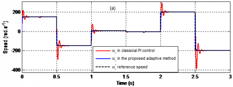
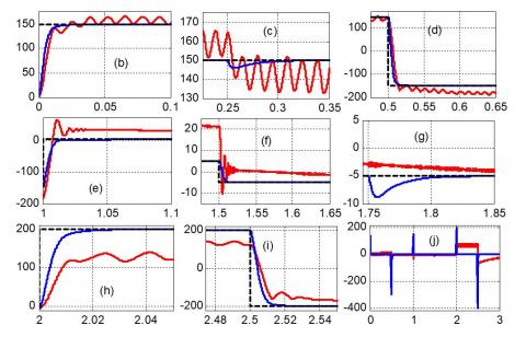
The Figure 3 shows the simulation results of the speed response without parameters uncertainty. From the Figure 3(a), we remark that the classical vector control and the proposed adaptive method follow the desired references. In the zoomed Figures 3(b) to 3(i) we can see that the motor actual speed with the proposed adaptive method closely follows the reference speed; at reversing speed and load torque application; without overshoot and undershoot and converges rapidly with shorter settling time (0.025s). It can be seen also that the motor follows the speed reference without oscillation in steady state time. In contrast, the settling time, the overshoot and the undershoot of the classical vector control are noted respectively as (0.125s), (50%) and (25%). In Figure 3(j), speed tracking errors $e_{\omega}$ is plotted, it is clear that the speed errors of the proposed method drop to zero rapidly than the classical vector control. This means that the PMSM tracks the reference speed trajectory with high accuracy in proposed control.
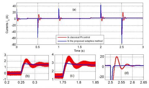
Furthermore, the Figures 4 and 5 show the control currents while the motor is running under load torque disturbance in the same mentioned conditions. As can be seen from the zoomed Figures 4(b) to 4(c) and 5(b) to 5(c), the proposed adaptive method follows the currents reference in steady state time without oscillations. On the other hand, the zoomed Figures 4(d) and 5(d) show the currents responses during speed reversing. We remark clearly that the proposed method tracks rapidly the currents reference.
Figure 3. Speed response under load torque disturbance only: (a) Speed response, (b) zoom around 0 s, (c) zoom around 0.25 s, (d) zoom around 0.5 s, (e) zoom around 1.0 s, (f) zoom around 1.5 s, (g) zoom around 1.75 s, (h)zoom around 2.0 s, (i) zoom around 2.5 s, (j) tracking errors
Figure 4. Evolution of the currents iq response under load torque disturbance: (a) currents response, (b) zoom around 0.25 s, (c) zoom around 1.75 s, (d) zoom around 2.5 s
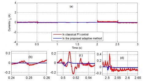
Figure 5. Evolution of the currents id response under load torque disturbance: (a) currents response, (b) zoom around 0.25 s, (c) zoom around 0.5 s, (d) zoom around 2.5 s
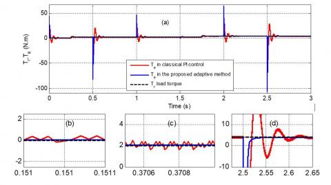
The Figures 6 presents the evolution of electrical torque responses under the same conditions mentioned above. We can also see that the proposed method follows the desired torque without oscillations in steady state time and drops rapidly to the desired reference during speed reversing.
Figures 7, 8, 9 and 10 show the simulations of uncertain PMSM, following the same desired trajectories, indicated above. In addition to mathematical uncertainty, perturbed PMSM parameters introduced in the control are set randomly to the following values: Increasing 300% in the stator resistance, 55% in the rotor moment of inertia and the friction, decreasing 25% in the stator inductances. The perturbed PMSM magnetic flux is expressed by the following function: $\varphi_{v}=-0.05 t+0.1546$ where t is the time.
The Figure 7 plots the desired and actual speed responses. As is shown in Figure 7(a), it is clear that the uncertain PMSM tracks precisely the reference speed trajectory with the proposed adaptive method, whereas the classical controller follows the reference quietly well at the beginning, after the application of the load torque of approximately $(2 N . m)$ it loses completely its performance. From the zoomed Figures 7(b) to 7(i) we can also see that the proposed method follows the desired speed without oscillations in steady state time and drops rapidly to the desired reference during speed reversing and load torque application. In addition, the Figure 7(j) displays the tracking errors. The tracking errors in steady state trends to zero with the proposed adaptive method but for the classical vector control the tracking errors rate is greater than 15%, 76% and 36% respectively in nominal, low and high speed simulations. Table 2 resume a qualitative comparison between proposed technique and classical vector control of PMSM.
Figure 6. Evolution of the torque responses under load torque disturbance only: (a) Torque responses, (b) zoom around 0.15s, (c) zoom around 0.37s, (d) zoom around 2.5s
Figure 7. Speed response in the presence of uncertainties: (a) Speed response, (b) zoom around 0s, (c) zoom around 0.25s, (d) zoom around 0.5s, (e) zoom around 1.0s, (f) zoom around 1.5s, (g) zoom around 1.75s, (h) zoom around 2.0s, (i) zoom around 2.5s, (j) tracking errors
Table 2. Performance comparison
|
|
Classical vector control |
Proposed technique |
|
Settling time (s) |
More than 0.045 |
Less than 0.015 |
|
overshoot |
More than 16% |
0% |
|
undershoot |
More than 16 % |
0% |
|
oscillation |
yes |
no |
|
stability |
no |
yes |
|
Static error |
More than 15% |
0 |
Figures 8 and 9 show respectively the evolution of the currents $i_{q}$ and $i_{d}$. The fluctuations that appear at the beginning and during speed inversion can be eliminated easily with the limiters. The simulation results for the currents trajectory tracking control at steady state time are shown in zoomed Figures 8(b) to 8(c) and 9(b) to 9(c). They indicate that in this situation the proposed adaptive method again has superior control performance to classical vector control. During the speed reversion, as can be seen from the zoomed Figures 8(d) and 9(d), it still has the best performance when the classical vector control degrades considerably.
Figure 8. Evolution of the currents iq response in the presence of uncertainties: (a) currents response, (b) zoom around 0.25s, (c) zoom around 1.5s, (d) zoom around 2.5s
Figure 9. Evolution of the currents id response in the presence of uncertainties: (a) currents response, (b) zoom around 0.25s, (c) zoom around 0.5s, (d) zoom around 2.5s
The Figure 10 plots the load torque disturbances variation and the electrical torque. Clearly, the zoomed Figures 10(b) and 10(c) show that the torque in the proposed method follow the load torque variation without ripples in the steady state time, whereas the classical vector control loses its reference and presents more ripples. As can be seen from Figure 10(d) the proposed adaptive method drops with short time to desired values and the classical vector control presents large ripples with long settling time during the speed reversing. Thus, the proposed adaptive method still gains better control performance over the classical vector control.
Figure 10. Evolution of the torque responses in the presence of uncertainties: (a) Torque responses, (b) zoom around 0.15s, (c) zoom around 0.37s, (d) zoom around 2.5s
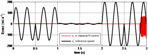
Once the speed and currents control system are designed with and without uncertainties, we proceed to prove the robustness of the proposed technique for uncertain PMSM by applying sinusoidal speed reference. The dynamic reference and actual speed response of the proposed adaptive method are given in Figure 11(a). We can observe that the disturbances rejection capacity of the proposed adaptive method leads to a good speed tracking performance. In addition, the Figure 11(b) presents the tracking errors. It shows that the asymptotic speed tracking objective is obtained with good accuracy under uncertainties.
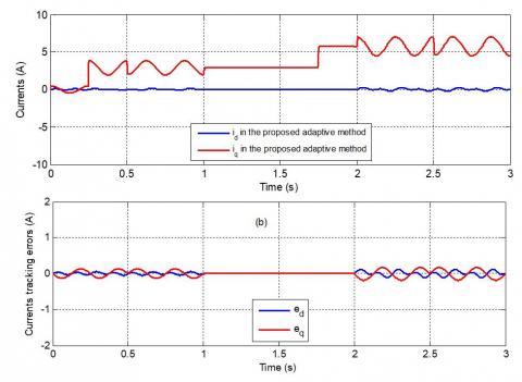
Furthermore, in the Figure 12 the evolution of the currents $i_{d}$ and $i_{q}$ and their tracking errors are presented. Since the reference speed trajectory is in sinusoidal form, the currents, $i_{d}$ and $i_{q}$ follow the same form as is shown in Figure 12(a), we note also that the current id is closely near to zero according to the control strategy. The Figure 12(b) shows that the tracking errors trends to zero with sinusoidal form due to the sinusoidal form of the speed reference.
The Figure 13 presents the load and electrical torques. We can observe from this figure that the electrical torque has also sinusoidal form with the average equal to the step of load torque disturbance. This is due to the sinusoidal form of the lumped disturbance and the uncertainty effect on the PMSM resulting from the sinusoidal form of the speed reference. As can be seen from this figure, precise control performance is reached during both transient and steady state times. In addition, we can observe that the tracking errors remain near to zero stably, in the presence of any uncertainty.
Figure 11. Speed response for sinusoidal reference in the proposed adaptive control in the presence of uncertainties: (a) Speed response and (b) speed tracking errors
Figure 12. Currents response in the proposed adaptive control in the presence of uncertainties: (a) Currents response and (b) currents tracking error
Figure 13. Evolution of the torque in the proposed adaptive control in the presence of uncertainties
Figure 14. Trajectories of the desired and actual speed with classical vector control in the presence of uncertainties
The proposed adaptive method, for its part, maintains its performance because of the adaptive compensation by reacting quickly to clear the errors occurred by the uncertainty. Whereas the classical vector control loses its reference completely in this case, as is demonstrated in Figure 14.
From the results of these simulations, it is seen clearly that the proposed adaptive method can suppress the uncertain behavior coming from mathematical modelling, parameters uncertainty and load torque disturbance in PMSM drive system and achieve a good tracking performance whatever the references of desired input signals.
This paper presents a robust speed-control strategy using stable and adaptive neural network compensators for the uncertain permanent magnet synchronous motor drives. The neural network compensators are based on the on-line parameter training methodology and they are designed to stabilize the PMSM despite of the uncertainties. The Hurwitz technique is used to determine the current controller gains, whereas the speed control is processed by PI controller. The stability of the closed-loop system is proven by using the Lyapunov function. Simulations are conducted to demonstrate the effectiveness of the proposed control scheme. Compared precisely to classical vector control, the obtained results show that all signals of the closed-loop system are tracked perfectly under the uncertainties conditions.
[1] Luo, Y., Chen, Y., Pi, Y. (2010). Cogging effect minimization in PMSM position servo system using dual high-order periodic adaptive learning compensation. ISA Transactions, 49(4): 479-488. https://doi.org/10.1016/j.isatra.2010.05.003
[2] Liu, H., Li, S. (2011). Speed control for PMSM servo system using predictive functional control and extended state observer. IEEE Transactions on Industrial Electronics, 59(2): 1171-1183. https://doi.org/10.1109/TIE.2011.2162217
[3] Quang, N.P., Dittrich, J.A. (2008). Vector control of three-phase AC machines (Vol. 2). Heidelberg: Springer.
[4] Lan, Y.H. (2018). Backstepping control with disturbance observer for permanent magnet synchronous motor. Journal of Control Science and Engineering. https://doi.org/10.1155/2018/4938389
[5] Chen, G., Zhou, Y., Gao, T., Zhou, Q. (2015). Unknown disturbance estimation for a PMSM with a hybrid sliding mode observer. Mathematical Problems in Engineering. https://doi.org/10.1155/2015/316360
[6] Lin, F.J., Chiu, S.L. (1998). Adaptive fuzzy sliding-mode control for PM synchronous servo motor drives. IEE Proceedings-Control Theory and Applications, 145(1): 63-72. https://doi.org/10.1049/ip-cta:19981683
[7] Wai, R.J. (2001). Total sliding-mode controller for PM synchronous servo motor drive using recurrent fuzzy neural network. IEEE Transactions on Industrial Electronics, 48(5): 926-944. https://doi.org/10.1109/41.954557
[8] Elmas, C., Ustun, O., Sayan, H.H. (2008). A neuro-fuzzy controller for speed control of a permanent magnet synchronous motor drive. Expert Systems with Applications, 34(1): 657-664. https://doi.org/10.1016/j.eswa.2006.10.002
[9] Maiti, S., Chakraborty, C., Sengupta, S. (2009). Simulation studies on model reference adaptive controller based speed estimation technique for the vector controlled permanent magnet synchronous motor drive. Simulation Modelling Practice and Theory, 17(4): 585-596. https://doi.org/10.1016/j.simpat.2008.08.017
[10] Rayd, H., El Idrissi, A.E.J., Zahid, N., Jedra, M. (2014). Robust emerged artificial intelligence speed controller for PMSM drive. 2014 Second World Conference on Complex Systems (WCCS), Agadir, Morocco, pp. 510-517. https://doi.org/10.1109/ICoCS.2014.7060952
[11] Yu, J., Gao, J., Ma, Y., Yu, H., Pan, S. (2010). Robust adaptive fuzzy control of chaos in the permanent magnet synchronous motor. Discrete Dynamics in Nature and Society. https://doi.org/10.1155/2010/269283
[12] Ran, J., Li, Y., Wang, C. (2018). Chaos and complexity analysis of a discrete permanent-magnet synchronous motor system. Complexity, 2018. https://doi.org/10.1155/2018/7961214
[13] Beniysa, M., El Idrissi, A. E. J., Bouajaj, A., Britel, M. R. (2020). A robust control of permanent magnet synchronous generator based wind energy conversion system via online-tuned artificial neural network compensators. International Conference on Artificial Intelligence & Industrial Applications, Meknes, Morocco, pp. 47-60. https://doi.org/10.1007/978-3-030-53970-2_5
[14] Aguilar-Mejía, O., Tapia-Olvera, R., Valderrabano-González, A., Rivas Cambero, I. (2016). Adaptive neural network control of chaos in permanent magnet synchronous motor. Intelligent Automation & Soft Computing, 22(3): 499-507. https://doi.org/10.1080/10798587.2015.1103971
[15] Poznyak, A.S., Sanchez, E.N., Yu, W. (2001). Differential neural networks for robust nonlinear control: identification, state estimation and trajectory tracking. World Scientific.
[16] Rivals, I., Personnaz, L. (1998). A recursive algorithm based on the extended Kalman filter for the training of feedforward neural models. Neurocomputing, 20(1-3): 279-294. https://doi.org/10.1016/S0925-2312(98)00021-6
[17] Bose, B.K. (2002). Modern Power Electronics and AC Drives. Prentice Hall PTR, Upper Saddle River, NJ 07458.
[18] Igelnik, B., Pao, Y.H. (1995). Stochastic choice of basis functions in adaptive function approximation and the functional-link net. IEEE transactions on Neural Networks, 6(6): 1320-1329. https://doi.org/10.1109/72.471375
[19] El-Sousy, F.F. (2014). Adaptive hybrid control system using a recurrent RBFN-based self-evolving fuzzy-neural-network for PMSM servo drives. Applied Soft Computing, 21: 509-532. https://doi.org/10.1016/j.asoc.2014.02.027
[20] de Jesús Rubio, J., Yu, W. (2007). Nonlinear system identification with recurrent neural networks and dead-zone Kalman filter algorithm. Neurocomputing, 70(13-15): 2460-2466. https://doi.org/10.1016/j.neucom.2006.09.004
[21] Lewis, F.L., Campos, J., Selmic, R. (2002). Neuro-fuzzy control of industrial systems with actuator nonlinearities. Society for Industrial and Applied Mathematics.
[22] Lewis, F.L. (2006). Neural network control of nonlinear discrete-time systems, CRC Press, Taylor & Francis Group.
[23] Sanchez, E.N., Ornelas-Tellez, F. (2013). Discrete-time inverse optimal control for nonlinear systems, CRC Press Taylor & Francis Group.
[24] Mohamad, S. (2008). Exponential stability preservation in discrete-time analogues of artificial neural networks with distributed delays. Journal of Computational and Applied Mathematics, 215(1): 270-287. https://doi.org/10.1016/j.cam.2007.04.009
[25] Luo, W., Zhong, K., Zhu, S., Shen, Y. (2014). Further results on robustness analysis of global exponential stability of recurrent neural networks with time delays and random disturbances. Neural Networks, 53: 127-133. https://doi.org/10.1016/j.neunet.2014.02.007
[26] Zhang, X.M., Han, Q.L. (2014). Global asymptotic stability analysis for delayed neural networks using a matrix-based quadratic convex approach. Neural Networks, 54: 57-69. https://doi.org/10.1016/j.neunet.2014.02.012
[27] Arik, S. (2014). An improved robust stability result for uncertain neural networks with multiple time delays. Neural Networks, 54: 1-10. https://doi.org/10.1016/j.neunet.2014.02.008
[28] Zhu, Y.H., Cheng, D.Z., Qin, H.S. (2007). Constructing common quadratic Lyapunov functions for a class of stable matrices. Acta Automatica Sinica, 33(2): 202-204. https://doi.org/10.1360/aas-007-0202
[29] Eghbal, N., Pariz, N., Karimpour, A. (2013). Discontinuous piecewise quadratic Lyapunov functions for planar piecewise affine systems. Journal of Mathematical Analysis and Applications, 399(2): 586-593. https://doi.org/10.1016/j.jmaa.2012.09.054
[30] King, C., Nathanson, M. (2006). On the existence of a common quadratic Lyapunov function for a rank one difference. Linear Algebra and its Applications, 419(2-3): 400-416. https://doi.org/10.1016/j.laa.2006.05.010
[31] Griggs, W.M., King, C.K., Shorten, R.N., Mason, O., Wulff, K. (2010). Quadratic Lyapunov functions for systems with state-dependent switching. Linear Algebra and Its Applications, 433(1): 52-63. https://doi.org/10.1016/j.laa.2010.02.011
[32] Dai, D., Hu, T., Teel, A.R., Zaccarian, L. (2009). Piecewise-quadratic Lyapunov functions for systems with dead zones or saturations. Systems & Control Letters, 58(5): 365-371. https://doi.org/10.1016/j.sysconle.2009.01.003
[33] El Idrissi, A.E.J., Zahid, N., Jedra, M. (2012). Optimized DTC by genetic speed controller and inverter based neural networks SVM for PMSM. In Second International Conference on the Innovative Computing Technology (INTECH 2012), Casablanca, Morocco, pp. 392-395. https://doi.org/10.1109/INTECH.2012.6457760
[34] Slotine, J.J.E., Li, W. (1991). Applied Nonlinear Control (Vol. 199, No. 1). Englewood Cliffs, NJ: Prentice Hall.