Zine El Abidine Harchouche* | Abdelkader Lousdad | Mothtar Zemri | Nabila Dellal | Foudil Khelil
© 2021 IIETA. This article is published by IIETA and is licensed under the CC BY 4.0 license (http://creativecommons.org/licenses/by/4.0/).
OPEN ACCESS
Friction Stir Welding (FSW) is a recent assembly process which has been developed at the British Welding Institute (TWI) at the beginning of the 90's. This welding process has gone a rapid development and an increasing success. Many remarkable industrial applications achieved mainly in spatial, aeronautical, automobile, railways, marine and naval industries.... The translation and the rotation of the tool during the FSW process generate the flow and plastic deformation of the material which had been often differently interpreted in contradictory manner. In this paper, an analytical model is proposed to describe the flow of matter in the vicinity of the FSW tool pin during the welding process. Analytical solutions are elaborated on the basis of conventional fluid mechanics theory which is used to solve the associated equation to the mentioned problem based on the Laurent's series (called also Laurent's development). The knowledge of the material flow around the tool pin can lead to a better understanding of the metallurgical phenomena which have a significant effect on the mechanical properties of the welded joint and allows a better description of the speed fields which is worth full for the thermal modelisation since the great part of the thermal power is generated by auto-heating energy. The results obtained on the effect of the speeds on the material flow are in good accordance with the experimental results found in the literature. The study highlights and gives a better understanding of the material flow phenomenon during the Friction Stir Welding process.
Friction Stir Welding (FSW), analytical model, matter, flow, Laurent series, tool pin
The knowledge of the matter flow trajectory in FSW process is neither perfect nor complete. The material flow depends mainly on the tool geometry. Many Authors have presented results by using different techniques of markers for welding of aluminum alloys. Such as the use of particles, steel balls, use of sheets, use of wire etc... Chronologically, the first, Colligan [1] had used steel balls of 0.38mm in diameter located at different initial positions in the plate before welding. They were positioned in grooves of 0.75mm X 0.3mm machined in the part before welding. These grooves can have a non-negligible effect on the flow of matter.
Another aluminum sheet of different material than the base metal has been inserted in different configurations before welding by the team of Reynolds et al. [2], Seide and Reynolds [3]. These alloys can recognize due to their different reactions to chemical attack. The conducted tests were of the same type in the two articles. Dickerson et al. [4], Guerra et al. [5], Schmidt et al. [6], Xu et al. [7] have used a sheet of copper. Sanders [8], Schneider and Nunes [9] have used a tungsten wire. Schneider et al. [10] used a tungsten wire or lead wire placed on the welding line at 1.3mm from the upper face of the sheets in order to put into evidence the movement of the particles in the thickness. In order to understand the role of the pin, Gratecap [11] has conducted experiments without complete penetration of the tool i.e., without full contact of the tool shoulder on the material. Striations had been put into evidence in the normal z planes.
They were interspaced by a distance equivalent to the feed per evolution. Liechty and Webb [12] by the quantification of the deposited matter, based on the final color of mixture, had put into evidence the difference between the path of the matter flow on the AS side and RS side. It seems the matter flow on the AS side is pushed forward then turn with tool before it can be deposited. Meanwhile the matter flow on the RS side is simply deposited on the back of the tool.
Moreover, by using six plasticine colors (three colors in the thickness), movements of matter flow have been observed in the thickness of the weld on the RS side. The obtained micro structural elements from FSW can reveal the path followed by the particles of matter in the observed zone.
These analyses were made by some Authors such as Sato et al. [13], Xu and Deng [7], Zhang et al. [14], Lee et al. [15], Liu and Nelson [16], Kumar et al. [17].
These research works allow to analyze the micro structural distribution and the nature of matter flow during the process. An improved Ultrasonic FSW (UVe FSW) has been developed by Liu and Wu [18]. The ultrasonic energy is directly transmitted in the weld zone near and before the tool in rotation via specially designed probe.
Hoyos et al. [19] presented a methodology for the elaboration of a semi-physical model based on the PBSM phenomenology applied for the evaluation of the rigidity of an aluminum alloy FSW joints.
In this paper an analytical approach is proposed which allow a complete description of the matter flow around the tool during the FSW process. The approach is based by considering two elementary speed fields namely a circumvention and circulation speeds. The analytical solutions are obtained based on the traditional fluid mechanics which is used to solve the associated equation to this problem using Laurent's series also known as Laurent's development.
After having developed the mathematical model of the matter flow two cases are considered for 7075 aluminum alloy: The first case considers different welding speed at a constant rotation speed and the second case considers different speed of rotation at a constant welding speed.
The results obtained by the proposed model are in good agreement with those obtained by Guedoiri [20] which describes the flow of aluminum alloy 7020-T6 by controlling the flow of the matter using copper thin sheets placed along and transversally with respect to the welding joint.
The results also are in good agreement with those obtained by Feulvarch et al. [21] who used a finite element of type P1+/P1 to model the flow of aluminum alloy 7075-T6 during the FSW process as well as with the results obtained by Bastier [22] who also used a finite element in order to simulate the flow of aluminum alloy 7075-T6 during the FSW process to estimate the mechanical residual state.
The aim of the present paper is the study of the matter flow in the most deformed zone generated by the FSW process for joining edge to edge sheets in order to see the material distribution after welding.
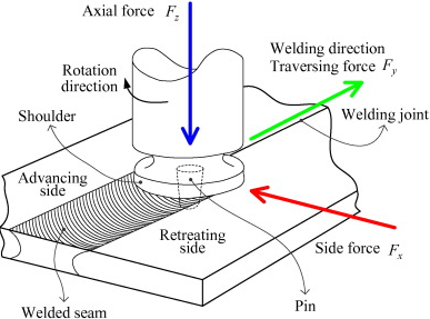
This welding process uses a specific tool made of two parts: the shoulder and the pin (Figure 1).
Figure 1. Schematic of FSW process
The weld can be obtained using 4 steps:
1. The approach phase: the tool is in rotation and penetrates the starting point of the weld under the effect of vertical translation movement until the contact of the shoulder with the upper face of the welding zone is reached.
2. The heating phase: the tool is in rotation without the vertical translation movement within a period of one to two seconds. The friction at the interface between the sheet and the tool shoulder generates heat which allows fusing the material to be welded.
3. The welding phase: The tool is in rotation and feed movements in order to perform the weld. During this period the matter is stirred by the pin and is deposed behind it.
4. The retraction phase: At the end of the welding phase the is the tool retracts upward and leaves a hole on the joined sheets. Figure 1 gives a schematic of the FSW process.
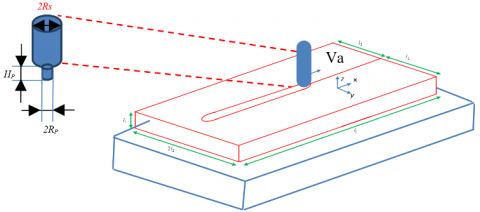
We consider two sheets of thickness l3 and dimensions l1 x 2l2 in the xy plan. The parts are fixed by clamping to avoid their spacing as shown in Figure 2.
The welded material moves in the x direction with a constant velocity Va. The FSW tool is made of steel has a flat ray of shoulder Rs (14mm), a cylindrical ray of pin RP (5mm) and a length of pin HP (3.95mm) [23].
Figure 2. Schematic illustration of the welded parts and the clamping system
The methodology proposed in this work consists in considering two elementary speed fields namely one field of circumvention speed and the other a circulation speed (Rotation around the tool pin).
4.1 Field of circumvention
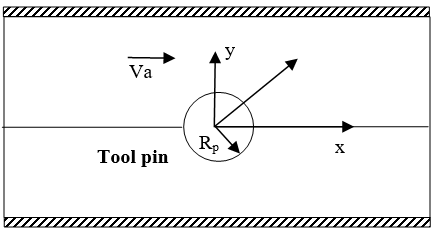
The first speed field corresponds to the circumvention speed (flow around the tool pin) when the welding advances.
In the first approach the problem is assimilated to an infinite cylinder (Figure 3) placed in a uniform speed field Va equals to the feed speed. The material is considered as perfect fluid, incompressible and irrotational. This speed field derives from a potential speed solution of Laplace's equation. This is invariant along the Z axis and must satisfy the two boundary conditions of the problem.
The speed of the tool pin equals to feed speed Va,
The normal component of speed is null at the pin contact.
Figure 3. Schematic illustration of the passage of the tool during friction stirs welding
The Navier-Stokes' equations are given as [24]:
$\rho \nabla v.v=-\nabla {{p}_{a}}+\mu \Delta v$ (1)
where, ρ, Pa, µ are respectively the density of the fluid, the hydrostatic pressure and the dynamic viscosity of the fluid.
In this problem the principle of conservation of mass can be described by the continuity equation under the following form:
$div(\rho \overrightarrow{v})+\frac{d\rho }{dt}=0$ (2)
When the volume stays constant under the action of the welding tool, it is considered as an incompressible fluid which can be expressed as:
$\rho =Cte$ (3)
Thus, the conservation of mass can be described by:
$div(\overrightarrow{v})=0$ (4)
We admit the characteristic equation f(z)=w which represents the complex potential of the speed of the fluid. This function is uniform in the domain K external to the pin section.
According to Laurent theorem [25]:
$w=u+vi=\sum\limits_{n=0}^{\infty }{{{a}_{n}}}{{z}^{n}}+\sum\limits_{n=0}^{\infty }{{{b}_{n}}}{{z}^{-n}}$ (5)
where, ${{a}_{n}}$ and ${{b}_{n}}$are the coefficient of Laurent series (see annex).
The solution to the problem must satisfies two boundary conditions:
The speed vector of the fluid, for z=∞, is directed along the x-axis and is equal to Va. The contour of the tool pin z=Rp is a part of the flow trajectory.
The speed is given by:
$\frac{\overline{dw}}{dz}=p+iq$ (6)
Thus, we have:
$\frac{\overline{dw}}{dz}=\sum\limits_{n=1}^{\infty }{n{{a}_{n}}}{{z}^{n-1}}-\sum\limits_{n=1}^{\infty }{n{{b}_{n}}}{{z}^{-n-1}}$ (7)
Since the development should be equal to Va at the infinite $\infty$, then $a_{n}=0$ for $\mathrm{n}>1$ and $a_{1}=V a$ because the infinite must be a regular point.
Consequently, the first condition leads to the following form of the characteristic equation f(z):
$w=a\,z+\sum\limits_{n=1}^{\infty }{{{b}_{n}}}{{z}^{-n}}$ (8)
Thus, the member b0 has eliminated knowing that its inclusion in the function f(z) has no effect on the values of the speed components p and q as well as on the function of the trajectory of the flow.
Assuming that $b_{n}=\rho_{n} e^{\alpha_{n} i}, z=r e^{\theta i}$ we obtain:
$u+vi=a\,r{{e}^{\theta i}}+\sum\limits_{n=1}^{\infty }{{{\rho }_{n}}}{{r}^{-n}}{{e}^{\left( {{\alpha }_{n}}-n\theta \right)i}}$ (9)
Thus, we find:
$u=ar\cos (\theta )+\sum\limits_{n=1}^{\infty }{{{\rho }_{n}}}{{r}^{-n}}\cos ({{\alpha }_{n}}-n\theta )$ (10)
$v=ar\sin (\theta )+\sum\limits_{n=1}^{\infty }{{{\rho }_{n}}}{{r}^{-n}}\sin ({{\alpha }_{n}}-n\theta )$ (11)
The second condition gives that v must maintain a constant value for r=Rp.
By deriving the second formula of Eqns. (10) and (11) with respect to θ and making r=Rp, we obtain:
$a{{R}_{p}}\cos (\theta )-\sum\limits_{n=1}^{\infty }{n{{\rho }_{n}}}{{R}_{p}}^{-n}\cos ({{\alpha }_{n}}-n\theta )=0$ (12)
Consequently, we have:
$\begin{align} & a{{R}_{p}}-{{\rho }_{1}}{{R}_{p}}^{-n}\cos {{\alpha }_{1}}=0,\,\,\,\,\,\,\,\,\,\,\,\,\,{{\rho }_{1}}{{R}_{p}}^{-n}\sin {{\alpha }_{1}}=0 \\ & n{{\rho }_{n}}{{R}_{p}}^{-n}\cos {{\alpha }_{n}}=n{{\rho }_{n}}{{R}_{p}}^{-n}\sin {{\alpha }_{n}}=0\,\,\,\,\,\,\,\,\,\,\,\,\,(n=2,3,....) \\\end{align}$ (13)
With $\rho_{n}=0(\mathrm{n}=2,3, \ldots), \rho_{1}=a R p^{2}, \alpha_{1}=0$.
The final form of the function of the trajectory of the fluid flow is:
$w={{V}_{a}}\,z+\frac{{{V}_{a}}\,{{R}_{p}}^{2}}{z}={{V}_{a}}\left( z+\frac{{{R}_{p}}^{2}}{z} \right)$ (14)
The functions of the speeds of the fluid u and v are expressed by the following formulae:
$u={{V}_{a}}\left( r+\frac{{{R}_{p}}^{2}}{r} \right)\cos \theta $
$v={{V}_{a}}\left( r-\frac{{{R}_{p}}^{2}}{r} \right)\sin \theta $ (15)
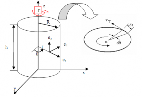
4.2 The speed of circulation
Figure 4. Field of the circulation speed
The second field is represented by the orthoradial vector of the material around the tool pin (i.e., the orthogonal vector to the radial vector and to the rotation axis). As shown on Figure 4, this axisymmetric field can be expressed in simple form in the cylindrical coordinate system. We consider a flow line which makes a closed loop. The speeds of all points are tangent to the curve of radius r. This flow line rotates with an angular speed w in a cylinder with OZ axis (perpendicular to the flow plane). We consider an element (ds) of this line.
We consider the characteristic function f(z):
$w=\frac{I}{2\pi i}Inz$ (16)
Also, by considering $z=r e^{\theta i}$, we determine the circulation speed fields u and v:
$u=\frac{I}{2\pi }\theta \,\,\,\,\,\,\,,v=-\frac{I}{2\pi }Inr$ (17)
The flow trajectories will be v=const or r=const, i.e., the concentric circles. The components p and q of the fluid speed are determined by the following formula:
$\frac{\overline{dw}}{dz}=p+iq=\frac{I}{2\pi r}{{e}^{i\left( \theta +\pi /2 \right)}}$ (18)
Thus, the value of the speed at all points of the circle of radius r is equal to $\frac{I}{2\pi r}$
Inversely proportional to r and directed in ccw direction. The fluid flow along the contour Γ surrounding the tool pin is:
$\int\limits_{C}{pdx}+qdy=\int\limits_{C}{du}=\frac{I}{2\pi r}\int\limits_{0}^{2\pi }{d\theta }=I$ (19)
Thus, the particles move along a circle in ccw direction and the flow speed is inversely proportional to the distance from the particle to the tool pin center.
4.3 Combination speeds of circumvention and circulation
By considering and adding the expressions of movements of sections (4.1) and (4.2), we obtain the fluid flow function generated around the tool pin with a speed Va and a circulation l as follows:
$w=\frac{I}{2\pi i}Inz+{{V}_{a}}\left( z+\frac{{{R}^{2}}}{z} \right)$ (20)
Consequently, the fluid flow functions u and v are expressed by the following formulae:
$u={{V}_{a}}\left( r+\frac{{{R}^{2}}}{r} \right)\cos \theta ,v={{V}_{a}}\left( r-\frac{{{R}^{2}}}{r} \right)\sin \theta +\frac{I}{2\pi r}$ (21)
The first speed field corresponds to the circumvention of the material around the tool pin when it advances. The second speed fields correspond to the orthoradial flow of the material around the tool pin.
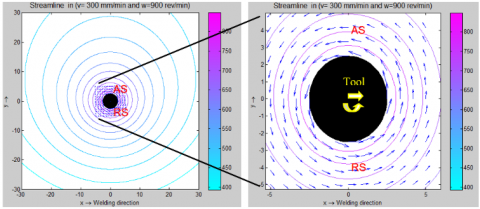
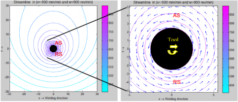
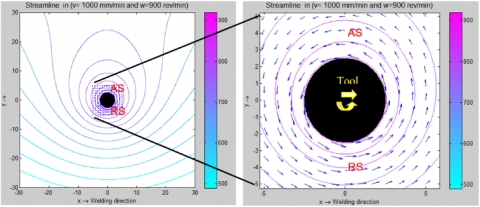
Figure 5 illustrates the distribution of the speed fields obtained by the proposed developed model.
The speed distribution is given in the transversal direction of aluminum 7075 materials assembly near the tool axis for four different speeds (100, 300, 600 and 1000 mm / min) with constant rotational speed of (900 rpm) in the cross-section perpendicular to the tool axis.
Figure 5 shows the total variation of the speed field by the integration of circumvention and circulation speed component expressed by Eqns. (15)-(21). Moreover, this speed components illustration shows the manner the field of circulation phenomenon dominates the field of circumvention speed and limits the penetration of the matter through the tool (kinematic incompatibility). These observations are common to all the figures.
(a)
(b)
(c)
(d)
Figure 5. Speed fields in the transverse direction in the plane of the welding junction during Friction Stir Welding process (With different welding speed and constant rotational speed)
The speed field intensity in the vicinity of the tool pin for different welding speeds (100, 300, 600 and 1000 mm/min) coincide quite well with the rotational speed. The symmetry of the speed field intensity appears in Figure 5 (a and b) for welding speeds of 100, and 300mm/min respectively. However, in the rest of the Figure 5 (c and d) for which the welding speeds are respectively 600 and 1000 mm/min, the symmetry cannot be visible.
This justifies the increase of the welding speed. Also, it can be noticed that the intensity of the speed field in the advance side takes lower values with respect of that of the retract tool side. Moreover, these figures put into evidence the presence of the rotating fluid with the tool before it can be expelled from the rotational zone. It appears that the particles make many turns before leaving the rotational zone around the tool. The obtained results are in agreement with those obtained by Guedoiri [20], Feulvarch et al. [21] and Bastier [22].
(a)
(b)
(c)
(d)
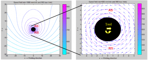
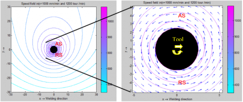
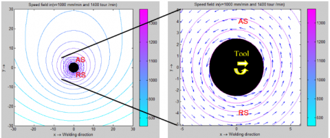
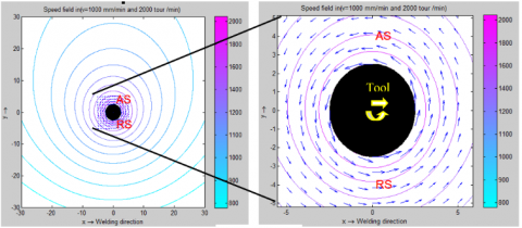
Figure 6. Fields of the speed in the transverse direction in the plan of junction of the welding during Friction Stir Welding process (With different rotational speed and constant welding speed)
Figure 6 shows the results of the speed fields distribution in the transversal direction of the welded 7075 aluminum assembly near the tool axis for four rotational speeds (900, 1200, 1400 and 2000 rpm with a constant welding speed of (1000 mm / min).
Figure 6 illustrates the total speed field variation including the circumvention and circulation components expressed by Eqns. (15)-(21). This speed of the total field comes up by including the circumvention and circulation components. The intensity of the speed near the tool pin is shown for different rotational speeds (900, 1200, 1400 and 2000 rpm) respectively.
As in the precedent case the axisymmetry appears in all the cases of the rotational speeds. However, it decreases when the rotational speed increases. It can also be noticed that the intensity of the speed field in the lateral advance side takes lower values with respect to the those of the tool pin in the retract side. The obtained results are in good agreement with those found in the literature.
In general, and in the case 1: different welding speeds with constant rotational speed and case 2: different rotational speeds and constant welding speed show that the variation of the welding speed and the rotational speed are important parameters with significant effect on the speed fields intensity around the tool pin.
The same observations are made as for the first case study and there exists a good agreement between the results obtained by our developed model and those obtained by Guedoiri [20], Feulvarch et al. [21] and Bastier [22].
The analytical solution in fluid mechanics has been presented for the description of the material flow during the Friction Stir Welding process. This analytical study had allowed a deep understanding of the process and the generated phenomena. The approach of modeling the phenomena allows reduction in experimental experiments and thus reduction in development time and costs. The obtained results show that:
1-The axisymmetric and speed fields intensities appear for all cases.
2- The intensity of the speed field of the material in the vicinity of the tool pin for different rotational and feed speeds are coincident i.e fall with the rotational speed of the pin.
3-The variation of the welding speed and tool rotational speed are important parameters with significant effect on the speed fields intensity around the tool pin.
4-The speed field intensity in lateral advance side takes lower values with respect to those of the tool pin retract side.
5-The study highlights and gives a better understanding of the material flow phenomenon during the Friction Stir Welding process.
|
l1 |
length of workpieces mm |
|
l2 |
width of workpieces mm |
|
l3 |
thickness of workpieces mm |
|
Rs |
ray of shoulder mm |
|
Rp |
ray of pin mm |
|
Hp |
length of pin mm |
|
Va |
welding speed mm. min-1 |
|
Greek symbols |
|
|
ρ |
density of the fluid, kg. m-3 |
|
Pa |
hydrostatic pressure N.m-2 |
|
µ |
dynamic viscosity of the fluid Pa.s |
|
Subscripts |
|
|
${{a}_{n}},{{b}_{n}}$ |
coefficient of Laurent series |
|
f(z) |
complex potential |
|
p,q |
components of the speed of the fluid |
Let $z \in K$, and let consider the couronne K1:r1< lz-zl0 < R1 containing point z where r1> r, R1<R as shown in Formula (A.1).
According to Cauchy integral theorem for a contour Γ= CR1++ Cr1- composed of circles with radius R1 and r1 respectively we have:
$\begin{align} & f(z)=\frac{1}{2\pi i}\int\limits_{{{C}_{{{R}_{1}}}}}{\frac{f(\zeta )d\zeta }{\zeta -z}}-\frac{1}{2\pi i}\int\limits_{{{C}_{{{r}_{1}}}}}{\frac{f(\zeta )d\zeta }{\zeta -z}}= \\ & \frac{1}{2\pi i}\int\limits_{{{C}_{{{R}_{1}}}}}{\frac{f(\zeta )d\zeta }{\left( \zeta -{{z}_{0}} \right)\left( 1-\frac{z-{{z}_{0}}}{\zeta -{{z}_{0}}} \right)}}-\frac{1}{2\pi i}\int\limits_{{{C}_{{{r}_{1}}}}}{\frac{f(\zeta )d\zeta }{\left( z-{{z}_{0}} \right)\left( 1-\frac{\zeta -{{z}_{0}}}{z-{{z}_{0}}} \right)}} \\ \end{align}$ (A.1)
Figure A.1. The couronne K1
The sery $\frac{1}{1-\frac{z-{{z}_{0}}}{\zeta -{{z}_{0}}}}={{\sum\limits_{n=0}^{\infty }{\left( \frac{z-{{z}_{0}}}{\zeta -{{z}_{0}}} \right)}}^{n}}$ uniformly converge with respect to $\zeta \in {{C}_{{{r}_{1}}}}$, as a geometrical sery of common ratio$q=\left| \frac{z-{{z}_{0}}}{\zeta -{{z}_{0}}} \right|\langle \,1$ , thus the sery$\frac{1}{1-\frac{\zeta -{{z}_{0}}}{z-{{z}_{0}}}}={{\sum\limits_{n=0}^{\infty }{\left( \frac{\zeta -{{z}_{0}}}{z-{{z}_{0}}} \right)}}^{n}}$ also converges uniformly with respect to $\zeta \in {{C}_{{{r}_{1}}}}$ for the same reason.
Then, if the two series are multiplied respectively by $\frac{f(\zeta )}{\zeta -{{z}_{0}}}$ and $\frac{f(\zeta )}{z-{{z}_{0}}}$, (the bonded functions on${{C}_{{{R}_{1}}}}$and${{C}_{{{r}_{1}}}}$)then, the obtained series will converge uniformly on the ${{C}_{{{R}_{1}}}}$and ${{C}_{{{r}_{1}}}}$ curves respectively. Consequently, the series${{\sum\limits_{n=0}^{\infty }{\frac{f(\zeta )}{\zeta -{{z}_{0}}}\left( \frac{z-{{z}_{0}}}{\zeta -{{z}_{0}}} \right)}}^{n}}$and ${{\sum\limits_{n=0}^{\infty }{\frac{f(\zeta )}{z-{{z}_{0}}}\left( \frac{\zeta -{{z}_{0}}}{z-{{z}_{0}}} \right)}}^{n}}$can be integrated along the curves ${{C}_{{{R}_{1}}}}$and ${{C}_{{{r}_{1}}}}$. Thus we obtain:
$\begin{align} & f(z)=\sum\limits_{n=0}^{\infty }{\frac{1}{2\pi i}\left( \int\limits_{{{C}_{{{R}_{1}}}}}{\frac{f(\zeta )d\zeta }{{{\left( \zeta -{{z}_{0}} \right)}^{n+1}}}} \right){{\left( z-{{z}_{0}} \right)}^{n}}+} \\ & \sum\limits_{-\infty }^{n=-1}{\frac{1}{2\pi i}\left( \int\limits_{{{C}_{{{r}_{1}}}}}{\frac{f(\zeta )d\zeta }{{{\left( \zeta -{{z}_{0}} \right)}^{n+1}}}} \right){{\left( z-{{z}_{0}} \right)}^{n}}} \\ \end{align}$ (A.2)
By taking any$\rho \left( r\langle \rho \langle R \right)$, it can be shown with Cauchy’s theorem that:
$\begin{align} & \int\limits_{{{C}_{{{R}_{1}}}}}{\frac{f(\zeta )d\zeta }{{{\left( \zeta -{{z}_{0}} \right)}^{n+1}}}}=\int\limits_{{{C}_{\rho }}}{\frac{f(\zeta )d\zeta }{{{\left( \zeta -{{z}_{0}} \right)}^{n+1}}}}; \\ & \int\limits_{{{C}_{{{r}_{1}}}}}{\frac{f(\zeta )d\zeta }{{{\left( \zeta -{{z}_{0}} \right)}^{n+1}}}}=\int\limits_{{{C}_{\rho }}}{\frac{f(\zeta )d\zeta }{{{\left( \zeta -{{z}_{0}} \right)}^{n+1}}}} \\ \end{align}$ (A.3)
By making:
${{a}_{n}}=\frac{1}{2\pi i}\int\limits_{{{C}_{\rho }}}{\frac{f(\zeta )d\zeta }{{{\left( \zeta -{{z}_{0}} \right)}^{n+1}}}},(n=0,\pm 1;\pm 2,....)$ (A.4)
where, $r\langle \rho \langle R$, then we can write:
$f(z)=\sum\limits_{n=-\infty }^{\infty }{{{a}_{n}}{{(z-{{z}_{0}})}^{n}}}$ (A.5)
[1] Colligan, K.J. (2010). Solid state joining fundamentals of friction stir welding. Failure Mechanisms of Advanced Welding Processes, 137-163. https://doi.org/10.1533/9781845699765.137
[2] Reynolds, A.P., Seidel, T.U., Simonsen, M. (2000). Visualisation of material flow in autogenous friction stir welds. Science and Technology of Welding Joining, 5(2): 120-124. https://doi.org/10.1179/136217100101538119
[3] Seidel, T.U., Reynolds, A.P. (2001). Visualization of the material flow in AA2195 friction-stir welds using a marker insert technique. Metallurgical and Materials Transactions A, 32(11): 2879-2884. https://doi.org/10.1007/s11661-001-1038-1
[4] Dickerson, T., Shercliff, H.R., Schmidt, H. (2003). A weld marker technique for flow visualization in friction stir welding. In 4th International Symposium on Friction Stir Welding, Park City, Utah, USA, pp. 1-12.
[5] Guerra, M., Schmidt, C., McClure, J.C., Murr, L.E., Nunes, A.C. (2003). Flow pattern during friction stir welding. Materials Characterization, 49(2): 95-101. https://doi.org/10.1016/S1044-5803(02)00362-5
[6] Schmidt, H.N.B., Dickerson, T.L., Hattel, J.H. (2006). Material flow in butt friction stir welds in AA2024T3. Acta Materialia, 54(4): 1199-1209. https://doi.org/10.1016/j.actamat.2005.10.052
[7] Xu, S., Deng, X. (2008). A study of texture patterns in friction stir welds. Acta Materialia, 56(6): 1326-1341. https://doi.org/10.1016/j.actamat.2007.11.016
[8] Sanders, J. (2007). Understanding the material flow path of the friction stir weld process. Master Thesis, Faculty of Missipi State University, USA.
[9] Schneider, J., Nunes, A.C. (2002). Thermo-mechanical processing in friction stir welds. The Minerals, Metals & Materials Society, 43-51.
[10] Schneider, J., Beshears, R., Nunes Jr, A.C. (2006). Interfacial sticking and slipping in the friction stir welding process. Materials Science and Engineering: A, 435-436: 297-304. https://doi.org/10.1016/j.msea.2006.07.082
[11] Gratecap, F. (2007). Contribution to friction stir welding process. Ph. D Thesis, School Centrale Nantes, France.
[12] Liechty, B.C., Webb, B.W. (2007). The use of plasticine as an analog to explore material flow in friction stir welding. Journal of Materials Processing Technology, 184(1-3): 240-250. https://doi.org/10.1016/j.jmatprotec.2006.10.049
[13] Sato, Y.S., Takauchi, H., Park, S.H., Kokawa, H. (2005). Characteristics of the kissing-bond in friction stir welded Al alloy 1050. Materials Science and Engineering: A, 405(1-2): 333-338. https://doi.org/10.1016/j.msea.2005.06.008
[14] Zhang, Z., Xiao, B., Ma, Z. (2013). Effect of segregation of secondary phase particles and “S” line on tensile fracture behavior of friction stir-welded 2024Al-T351 joints. Metallurgical and Materials Transactions, 44: 4081-4097. https://doi.org/10.1007/s11661-013-1778-8
[15] Lee, Y.R., No, K., Yoon, J.H., Yoo, J.T., Lee, H.S. (2016). Investigation of microstructure in friction stir welded Al-Cu-Li alloy. Key Engineering Materials, 705: 240-244. https://doi.org/10.4028/www.scientific.net/KEM.705.240
[16] Liu, F.C., Nelson, T.W. (2016). In-situ material flow pattern around probe during friction stir welding of austenitic stainless steel. Materials and Design, 110: 354-364. https://doi.org/10.1016/j.matdes.2016.07.147
[17] Kumar, R., Pancholi, V., Bharti, R.P. (2018). Material flow visualization and determination of strain rate during friction stir welding. Journal of Materials Processing Tech., 255: 470-476. https://doi.org/10.1016/j.jmatprotec.2017.12.034
[18] Liu, X.C., Wu, C.S. (2015). Material flow in ultrasonic vibration enhanced friction stir welding. Journal of Materials Processing Technology, 225: 32-44. https://doi.org/10.1016/j.jmatprotec.2015.05.020
[19] Hoyos, E., López, D., Alvarez, H. (2016). A phenomenologically based material flow model for friction stir welding. Materials and Design, 111: 321-330. https://doi.org/10.1016/j.matdes.2016.09.009
[20] Guedoiri, A. (2012). A contribution to the modeling and numerical simulation of friction stir welding. Ph.D Thesis. Arts et Metiers Institute of Technology, France.
[21] Feulvarch, E., Robin, V., Boitout, F., Bergheau, J.M. (2007). A 3D finite element modelling for thermofluid flow in friction stir welding. In: Cerjack H., Bhadeshia H.K.D.H., Kozeshnik E. (eds) Mathematical modelling of weld phenomena 8, Graz University of Technology, German.
[22] Bastier, A. (2006). Modelling of friction stir welding of aluminium alloys. Ph.D Thesis, Polytechnic Institute of Paris.
[23] Harchouche, Z., Zemri, M., Lousdad, A. (2019). Analytical modeling and analysis of the matter flow during friction stir welding. Solid State Phenomena, 297: 1-16. https://doi.org/10.4028/www.scientific.net/SSP.297.1
[24] Heuzé, T. (2011). Modelling fluid/solid couplings in high temperature assembly processes. Ph.D Thesis, University of Pierre and Marie Curie, Paris, 193: 183-193.
[25] Baddari, K., Abbassov, A. (2015). Practical theory of functions of a complex variable. Academic Publications Officer, Algeria.