Farid Belouahchi* | Elkheir Merabet
© 2020 IIETA. This article is published by IIETA and is licensed under the CC BY 4.0 license (http://creativecommons.org/licenses/by/4.0/).
OPEN ACCESS
This paper describes a new Direct Torque Control (DTC) scheme to the synthesis of controllers based on the theory of synergetic control (SC) for two level inverter fed double star induction motor (DSIM) drive. The controllers’ synthesis method is totally analytical, and is based on non-linear models of the DSIM. The proposed synergetic control scheme requires creation of the space attractors and artificial manifolds that reflect the desirable operating modes of the DSIM. The combination between the DTC and the SC laws provides asymptotic stability with respect to the required operating regimes, reduces the THD of stator currents, invariance to external disturbances, and robustness to variation of DSIM parameters. The performance of the proposed approach has been tested under different operating conditions. With respect to their dynamic characteristics, synergetic controllers (SCs) are superior to the existing types of PI, Sliding Mode (SM) and Fuzzy Logic (FL) controllers.
(DSIM) double star induction motor, (SMC) sliding mode control, (FLC) fuzzy logic control, (SC) synergetic control, (THD) total harmonic distortion, Lyapunov’s theory
In recent years, the double star induction motor has been largely replaced asynchronous machines, it is the dominant technology used today [1, 2], indeed, this priority due to numerous factors such as, great power, power segmentation, minimizing torque ripples, high reliability, ruggedness, low cost and minimal loss...etc. [3, 4].This type of machines is constituted by two windings shifted between them by an angle of 30 degrees. These windings are usually fed by a six-phase inverter supply in variable speed. The main benefits of DSIM are higher torque density, higher efficiency, reduced harmonic content of the DC link voltage [5].
Currently, several moderns control techniques have been proposed to control the double star induction motors such as, direct torque control, feedback control, vector control, adaptive control …etc. [6]. Among these approaches, the DTC technique has been proposed by Takahashi and Depenbrock in 1985 which considered a solution for the problems of vector control [6]. This technique does not look the voltages to be applied to the machine, but the best switching state of the inverter to satisfy the user's requirements [7]. The method supplies direct control of the stator flux and torque and gives a systematic solution to improve the operating characteristics of the motor and the voltage source inverter. This method is not a complex structure compared to field orientation control (FOC) [8], DTC gives a very fast and accurate torque response, simple to introduce, torque, flux ripples and acoustic noise produce significant stable state [9]. The principal advantage of DTC is not requiring speed or position encoders and uses the measured voltage and current only. Flux, torque, and speed are estimated [10]. Direct torque control allows fast and efficient control of the stator flux and torque by optimal selection of the inverter switch states in each sampling period. The additional inverter is available for multiphase machines, allows greater flexibility in their selection and therefore more narrow adjustment of stator flux and torque. The control is realized by only eight possible inverter states in three phases on the other hand at several of inverter states means that a more elaborate selection criterion is required. For this reason, a small research was presented on a switching-table-based direct torque control of multiphase drives [7]. Due to the parametric sensitivity of PID regulator, minimal research has been done to avoid this inconvenient such as in the papers [11-13], to solve these problems, the use of a non-linear technique is essential, among them the fuzzy logic, which considered one of the most successful artificial intelligence technique for controlling nonlinear systems, sliding mode control (SMC) which ensuring good system and robustness to external disturbance and parametric variations [14-16].
Regardless all these advantages of SMC control the major inconvenient is the phenomenon of chattering. Therefore, to solve this problem, a new technique for controlling nonlinear systems called synergetic approach has been proposed by Yu et al. [17, 18]. The works used this kind of controller demonstrate that it offers good robustness with respect for the possibility of parametric variation and also high efficiency, design simplicity and flexibility of synergetic controller [18], these advantages explicate the need of applying this kind of controller for the DSIM which used in higher power applications [18].
In this paper, a direct torque control (DTC) scheme based on synergetic approach for the two-level inverter fed double star induction motor (DSIM) drive has been proposed. The purpose of this work is to exploit the benefits of DTC control and to make a combination between DTC control and synergetic approach to obtain more performances of control applied. The performances of the proposed approach have been tested under different operating conditions. To illustrate the effectiveness and the superiority of the proposed approach, a comparative study has been done with PI, sliding mode control (SMC) and fuzzy logic control (FLC) and by using MatLab/Simulink the simulation results are presented and analyzed.
The structure of present paper is classified as follow: The description and the modeling of the DSIM have been presented in section 2. The control strategy applied to DSIM (DTC) is set in section 3. The design of synergetic control of DSIM is developed in section4. Moreover, the simulation results are discussed on Matlab/Simulink for the proposed control scheme in section 5. Finally, a general conclusion summarizes this work.
The stators and rotor voltage equations are expressed by:
$\begin{align} & \left[ {{v}_{s1}} \right]=\left[ {{R}_{s1}} \right]\left[ {{i}_{s1}} \right]+\frac{d}{dt}\left[ {{\phi }_{s1}} \right] \\ & \left[ {{v}_{s2}} \right]=\left[ {{R}_{s2}} \right]\left[ {{i}_{s2}} \right]+\frac{d}{dt}\left[ {{\phi }_{s2}} \right] \\ & \left[ {{v}_{r}} \right]=\left[ {{R}_{r}} \right]\left[ {{i}_{r}} \right]+\frac{d}{dt}\left[ {{\phi }_{r}} \right] \\ \end{align}$ (1)
where, vs1, vs2, vr and is1, is2, ir are stator and rotor voltage and current vectors.
The voltage, current and flux vectors are:
For star1:
$\begin{align} & \left[ {{v}_{s1}} \right]={{\left[ \begin{matrix} {{v}_{as1}} & {{v}_{bs1}} & {{v}_{cs1}} \\\end{matrix} \right]}^{T}} \\ & \left[ {{i}_{s1}} \right]={{\left[ \begin{matrix} {{i}_{as1}} & {{i}_{bs1}} & {{i}_{cs1}} \\\end{matrix} \right]}^{T}} \\ & \left[ {{\phi }_{s1}} \right]={{\left[ \begin{matrix} {{\phi }_{as1}} & {{\phi }_{bs1}} & {{\phi }_{cs1}} \\\end{matrix} \right]}^{T}} \\ \end{align}$ (2)
For star2:
$\begin{align} & \left[ {{v}_{s2}} \right]={{\left[ \begin{matrix} {{v}_{as2}} & {{v}_{bs2}} & {{v}_{cs2}} \\\end{matrix} \right]}^{T}} \\ & \left[ {{i}_{s2}} \right]={{\left[ \begin{matrix} {{i}_{as2}} & {{i}_{bs2}} & {{i}_{cs2}} \\\end{matrix} \right]}^{T}} \\ & \left[ {{\phi }_{s2}} \right]={{\left[ \begin{matrix} {{\phi }_{as2}} & {{\phi }_{bs2}} & {{\phi }_{cs2}} \\\end{matrix} \right]}^{T}} \\ \end{align}$ (3)
For rotor:
$\begin{align} & \left[ {{v}_{r}} \right]={{\left[ \begin{matrix} {{v}_{ar}} & {{v}_{br}} & {{v}_{cr}} \\\end{matrix} \right]}^{T}} \\ & \left[ {{i}_{r}} \right]={{\left[ \begin{matrix} {{i}_{ar}} & {{i}_{br}} & {{i}_{cr}} \\\end{matrix} \right]}^{T}} \\ & \left[ {{\phi }_{r}} \right]={{\left[ \begin{matrix} {{\phi }_{ar}} & {{\phi }_{br}} & {{\phi }_{cr}} \\\end{matrix} \right]}^{T}} \\ \end{align}$ (4)
The DSIM dynamic equations in the reference d-q can be writing as follow:
$\begin{align} & {{V}_{ds1}}={{R}_{s1}}{{i}_{ds1}}+\frac{d{{\phi }_{ds1}}}{dt}-{{\omega }_{s}}{{\phi }_{qs1}} \\ & {{V}_{qs1}}={{R}_{s1}}{{i}_{qs1}}+\frac{d{{\phi }_{qs1}}}{dt}+{{\omega }_{s}}{{\phi }_{ds1}} \\ & {{V}_{ds2}}={{R}_{s2}}{{i}_{ds2}}+\frac{d{{\phi }_{ds2}}}{dt}-{{\omega }_{s}}{{\phi }_{qs2}} \\ \end{align}$
$\begin{align} & {{V}_{qs2}}={{R}_{s2}}{{i}_{qs2}}+\frac{d{{\phi }_{qs2}}}{dt}+{{\omega }_{s}}{{\phi }_{ds2}} \\ & {{V}_{dr}}=0={{R}_{r}}{{i}_{dr}}+\frac{d{{\phi }_{dr}}}{dt}-({{\omega }_{s}}-{{\omega }_{r}}){{\phi }_{qr}} \\ & {{V}_{qr}}=0={{R}_{r}}{{i}_{qr}}+\frac{d{{\phi }_{dr}}}{dt}+({{\omega }_{s}}-{{\omega }_{r}}){{\phi }_{dr}} \\ \end{align}$ (5)
The fluxes equations are:
$\begin{align} & {{\phi }_{ds1}}={{L}_{s1}}{{i}_{ds1}}+{{L}_{m}}({{i}_{ds1}}+{{i}_{ds2}}+{{i}_{dr}}) \\ & {{\phi }_{qs1}}={{L}_{s1}}{{i}_{qs1}}+{{L}_{m}}({{i}_{qs1}}+{{i}_{qs2}}+{{i}_{qr}}) \\ & {{\phi }_{ds2}}={{L}_{s2}}{{i}_{ds2}}+{{L}_{m}}({{i}_{ds1}}+{{i}_{ds2}}+{{i}_{dr}}) \\ & {{\phi }_{qs2}}={{L}_{s2}}{{i}_{qs2}}+{{L}_{m}}({{i}_{qs1}}+{{i}_{qs2}}+{{i}_{qr}}) \\ & {{\phi }_{dr}}={{L}_{r}}{{i}_{dr}}+{{L}_{m}}({{i}_{ds1}}+{{i}_{ds2}}+{{i}_{dr}}) \\ & {{\phi }_{qr}}={{L}_{r}}{{i}_{qr}}+{{L}_{m}}({{i}_{qs1}}+{{i}_{qs2}}+{{i}_{qr}}) \\ \end{align}$ (6)
For studying the dynamic behavior, the following equation of movement was added:
$J\frac{d{{\Omega }_{r}}}{dt}={{T}_{em}}-{{T}_{L}}-{{K}_{f}}{{\Omega }_{r}}$ (7)
The model of the DSIM has been completed by the expression of the electromagnetic torque Tem given below:
${{T}_{em}}=P\frac{{{L}_{m}}}{{{L}_{m}}+{{L}_{r}}}({{\phi }_{dr}}({{i}_{qs1}}+{{i}_{qs2}})-{{\phi }_{qr}}({{i}_{ds1}}+{{i}_{ds2}}))$ (8)
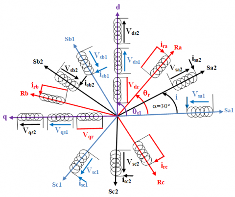
Figure 1. Schematic representation of DSIM in abc and d-q reference
A schematic representation of the stator and rotor windings axis of double star induction motor in the synchronous reference frame (d, q) has been illustrated in Figure 1.
Takahachi and Noguchi [19] proposed the classical DTC which based on the following algorithm:
Divide the time domain into short-lived duration.
Measure line currents and phase voltages of the DSIM for each clock struck.
Through the measurement of line current and stator flux the stator flux components and the electromagnetic torque have been estimated.
Input of the used three level hysteresis comparator is the error between the estimated torque and the reference one, this comparator generates at its output the value of +1 to increase the flux and 0 to reduce it and thus increasing the torque -1, it reduces this flux and 0 to keep it constant in a band.
For the two level of the hysteresis comparator, its input is the error between the estimated stator flux magnitudes and its reference; its output gives the value +1 to increase the flux and 0 to reduce it.
The state of the switches to determine the operating sequences of the inverter is selected through the switching table.
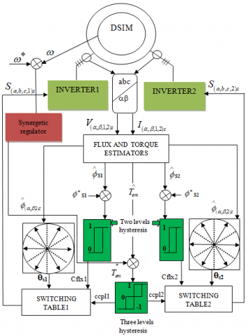
Figure 2 illustrates the synoptic diagram of the DTC of DSIM. In addition, Table 1 shows the sequences corresponding to the position of the stator flux vector to the different sectors.
Figure 2. Block diagram of DSIM speed synergetic under DTC
The expression of the stator flux is given by the following equations:
$\begin{align} & {{\phi }_{s\alpha 1,2}}=\int\limits_{0}^{t}{({{V}_{s\alpha 1,2}}-{{R}_{s}}}{{i}_{s\alpha 1,2}})dt \\ & {{\phi }_{s\beta 1,2}}=\int\limits_{0}^{t}{({{V}_{s\beta 1,2}}-{{R}_{s}}}{{i}_{s\beta 1,2}})dt \\ \end{align}$ (9)
where, Vsa1.2 and Vsb1.2 are the estimated components of the stator vector voltage. They are expressed from the model of the inverter.
Table 1. Switch table of DTC control
|
Corrector |
Cflx |
Ccpl |
1 |
2 |
3 |
4 |
5 |
6 |
|
2 levels |
1 |
1 |
V2 |
V3 |
V4 |
V5 |
V6 |
V1 |
|
0 |
V7 |
V0 |
V7 |
V0 |
V7 |
V0 |
||
|
3 levels |
-1 |
V6 |
V1 |
V2 |
V3 |
V4 |
V5 |
|
|
2 levels |
0 |
1 |
V3 |
V4 |
V5 |
V6 |
V1 |
V2 |
|
3 levels |
0 |
V7 |
V0 |
V7 |
V0 |
V7 |
V0 |
|
|
-1 |
V5 |
V6 |
V1 |
V2 |
V3 |
V4 |
Generally, the dynamic representation of nonlinear systems is as follow [17, 20, 21]:
$\dot{X}=f\left( X,u,t \right)$ (10)
where, x represents the system state vector, u represents the control vector and t is time.
The design of synergetic control is obtained into two steps:
The first step is the determination of macro-variable defined as a function of the state variables of the system.
$\Psi =\psi \left( X,t \right)$ (11)
where, $\Psi$ is the macro-variable and $\psi$ (X, t) a function chosen by the user. For study the different constraints on the system, we change the macro-variable according to the constraint to study, the system will be forced to operate on the manifold by the used control $\Psi$= 0.
The second step is a determination of the desired dynamic evolution of the macro-variable to the manifold $\Psi$= 0 by an equation; this equation has the following general form [22, 23]:
$T\dot{\psi }+\psi =0$ (12)
With T>0.
where, T is the control parameter, which specifying the convergence speed to the manifold specified by the macro-variable.
The solution of the Eq. (8) gives the following function:
$\psi \left( t \right)={{\psi }_{0}}\mathop{e}^{-\frac{t}{\tau }}$ (13)
Taking into consideration the chain of differentiation, which is given by Medjbeur et al. [21-23]:
$\frac{d\psi \left( X,t \right)}{dt}=\frac{d\psi \left( X,t \right)}{dX}\frac{dX}{dt}$ (14)
Substitution of the Eqns. (11) and (12) in (14) we find:
$\frac{d\psi \left( X,t \right)}{dt}f\left( X,u,t \right)+\psi \left( X,t \right)=0$ (15)
The solution of equation (11) for “u” gives us the following control law as follow [17, 20, 21]:
$u=g\left( X,\psi \left( X,t \right),T,t \right)$ (16)
From the Eq. (12), it is clear that the control does not only relate with the variable state of the system, but also with the macro-variable and the control parameter T. It means that, the choose of macro-variable appropriate and specific control parameters T by the designer determine the characteristics of the controller. In the synthesis of synergic controller shown above, it noticed that the latter deals with the non-linear system and a linearization or simplification of the model is not necessary, as is often the case of traditional control approaches.
Generally, the use of parameters, state variables and time of convergence of the system allows us to develop the laws of control. If we use in our research one macro-variable which is a linear function of the mechanical state variables, it generally has the following form:
${{\psi }_{1}}=\alpha {{x}_{1}}+\beta {{x}_{2}}$ (17)
where,
$\begin{align} & {{x}_{1}}={{\omega }_{r\_ref}}-{{\omega }_{r}} \\ & {{x}_{2}}={{\phi }_{r\_ref}}-{{\phi }_{r}} \\ \end{align}$ (18)
y1 must satisfy the following equation:
$T{{\dot{\psi }}_{1}}+\psi =0$ T>0 (19)
Substitution of Eqns. (13) and (14) into (15) we get:
$\begin{align} & T\left( \alpha {{{\dot{x}}}_{1}}+\beta {{{\dot{x}}}_{2}} \right)+\alpha {{x}_{1}}+\beta {{x}_{2}}=0 \\ & -T\left( \alpha \frac{d{{\omega }_{r}}}{dt}+\beta \frac{d{{\phi }_{r}}}{dt} \right)+\alpha \left( {{\omega }_{r\_ref}}-{{\omega }_{r}} \right)+\beta \left( {{\phi }_{r\_ref}}-{{\phi }_{r}} \right)=0 \\ \end{align}$ (20)
We have:
$\begin{align} & \frac{d{{\omega }_{r}}}{dt}=\frac{1}{J}\left( P{{T}_{em}}-P{{T}_{L}}-{{k}_{f}}{{\omega }_{r}} \right) \\ & \frac{d{{\phi }_{r}}}{dt}=\frac{{{R}_{r}}}{{{L}_{r}}+{{L}_{m}}}{{\phi }_{r}}+\frac{{{R}_{r}}{{L}_{m}}}{{{L}_{r}}+{{L}_{m}}}\left( {{i}_{ds1}}+{{i}_{ds2}} \right) \\ \end{align}$ (21)
Replacing Eq. (17) into Eq. (16) we get:
$-T\left( \alpha \frac{1}{J}\left( P{{T}_{em}}-P{{T}_{L}}-{{k}_{f}}{{\omega }_{r}} \right)+\beta \frac{d{{\phi }_{r}}}{dt} \right)+\alpha \left( {{\omega }_{r\_ref}}-{{\omega }_{r}} \right)+\beta \left( {{\phi }_{r\_ref}}-{{\phi }_{r}} \right)$ (22)
From Eq. (18) we obtained the following control law:
${{T}_{em}}=\frac{J}{TP\alpha }\left( \alpha \left( {{\omega }_{r\_ref}}-{{\omega }_{r}} \right)+\beta \left( {{\phi }_{r\_ref}}-{{\phi }_{r}} \right)-T\beta \frac{d{{\phi }_{r}}}{dt} \right)+{{T}_{L}}+\frac{{{k}_{f}}}{P}{{\omega }_{r}}$ (23)
where, $=\alpha, \beta$ and T are the controller parameters.
The control of the drive system has been tested by simulation under DTC scheme using synergetic controller; the results are performed in this paper by using MATLAB/SIMULINK. The used double star induction motor has the following parameters, the nominal power Pn is 4.5kw, nominal voltage Vn is 220V, stator resistances Rs1 and Rs2 are 3.72 Ohm, rotor resistance Rr is 2.12 Ohm, mutual inductance Lm is 0.3672H, rotor inductance Lr is 0.006H, moment of inertia J is 0.0662kg.m2, and friction coefficient Kf is 0.001.The simulation results have been obtained for two tests conditions in addition to the robustness tests. The performances of the proposed approach have been compared with PI, sliding mode control (SMC) and fuzzy logic control (FLC).
6.1 Tracking the performance of synergetic controller under two different tests and robustness tests
6.1.1 Reference tracking test
Two different tests are applied:
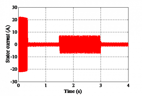
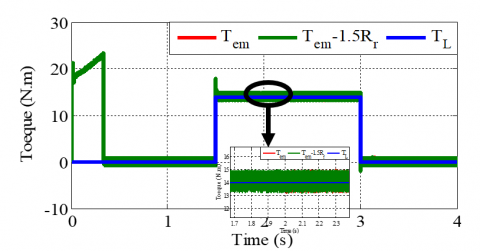
The first test is the no load start then under load with load torque is TL= 14 N.m and reference speed are wref=100rd/sec.
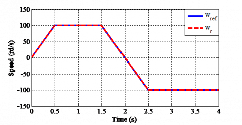
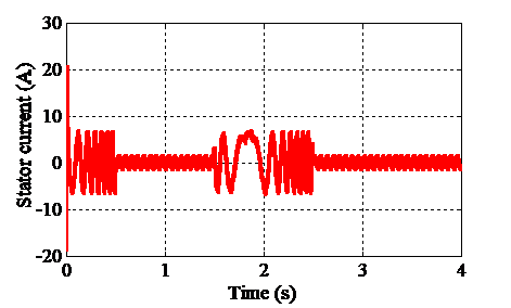
The second test is the no load start with inversion of reference speed from 100rd/sec to -100rd/sec, for all tests the reference flux is 1Wb.
Figure 3 and 4 respectively presents different responses of electromagnetic torque, speed, stator flux and stator current for the first test and the second test.
i. FIRST TEST
(a)
(b)
(c)
(d)
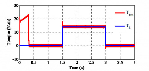
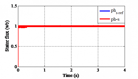
Figure 3. Torque, speed, stator flux and current responses for the first test
Figure 3 illustrates the simulation results of the first test, the electromagnetic torque has the same form of the load torque which shows that it compensates the load torque and the friction in the established regime (Figure 3(a)), the speed reaches the reference speed at t=0.3s and follows it perfectly, it also noticed that the speed controller rejects the load disturbance quickly (Figure 3(b)), the stator current has a peak value at the start up of 21A, in the presence of load its peak value is 7A and 1.5A in the absence of theme (no load) (Figure 3(d)).
ii. SECOND TEST
(a)
(b)
(c)
(d)
Figure 4. Torque, speed, stator flux and current responses for the second test
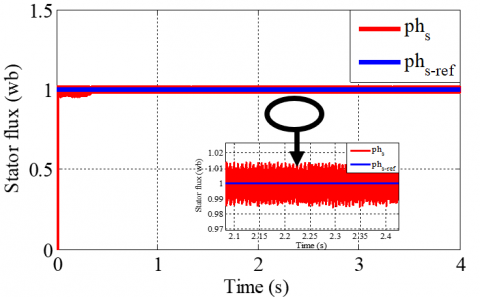
Figure 4 represents the simulation results of the second test, the speed follows its reference and reverses such as it reaches the value -100rd/s at t=2.5s Figure 4(b), the reversal of direction of rotation from t=1.5s to t=2.5s leads to a negative electromagnetic torque of -14N.m (Figure 4(a)), the stator current amplitude is similar to that the startup (Figure 4(d)), in all the two tests the stator flux tracked its reference perfectly (Figure 3(c) and 4(c)).
6.1.2 Robustness test
The robustness tests are done as follow:
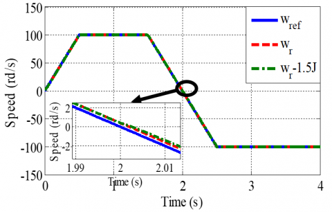
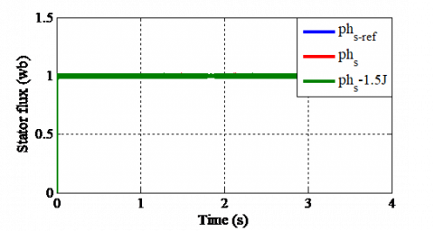
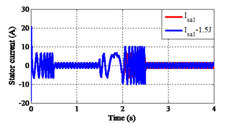
Figure 5, 6 and 7 respectively present different responses of electromagnetic torque, speed, stator flux and stator current for the robustness tests (variation of rotor resistance, load torque and inertia moment).
(a)
(b)
(c)
(d)
Figure 5. Torque, speed, stator flux and current responses for an increase of rotor resistance by 50%
Figure 5 exhibits the simulation results of the first robustness test which is an increase of rotor resistance by 50%, the simulation results of this test show that the sensitivity of the speed due to the variation of the rotor resistance is not apparent (Figure 5(b)) and we have a small change in the torque, the flux and the stator current during this variation (Figures 5(a), 5(c) and 5(d)).
Figure 6 reveals the simulation results of the second test of robustness which is an increase of load torque by 50%, the simulation results of this test demonstrate that the electromagnetic torque follows the load torque despite its variation (Figure 6(a)), the latter creates a change in the stator current due to the relation between the current and the electromagnetic torque (Figure 6(d)), for speed and stator flux, any changes have been observed due to this variation (Figures 6(b) and 6(c)).
Figure 7 shows the simulation results of the third test of robustness which is an increase of inertia moment by 50%, the speed follows its reference with any changes due to variation of inertia moment (Figure 7(b)) and we have a small variation of stator flux (Figure 7(c)), for the electromagnetic torque and the stator current, it noticed that it increased during this variation thanks to the relation between the electromagnetic torque, the stator current and the inertia moment (Figures 7 (a) and 7(d)).
(a)
(b)
(c)
(d)
Figure 6. Torque, speed, stator flux and current responses for an increase of load torque by 50%
(a)
(b)
(c)
(d)
Figure 7. Torque, speed, stator flux and current responses for an increase of inertia moment by 50%
6.2 Assessment the performance of synergetic controller with others techniques
In this part of simulation, the performances of the used approach (synergetic) have been compared with others techniques under two different tests:
6.2.1 Reference tracking test
In this section, the form of reference speed is chosen as a stair curve with amplitude of 100rd/s, -100rd/s, 0rd/s and 50rd/s.
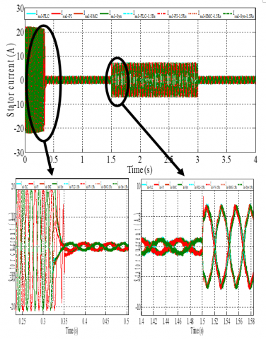
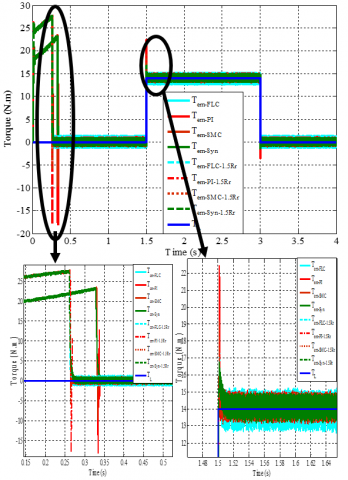
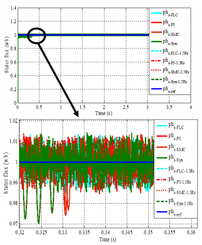
Figure 8 presents different responses of speed, torque, stator current and stator flux for the reference tracking test.
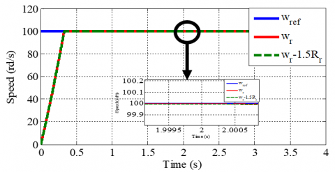
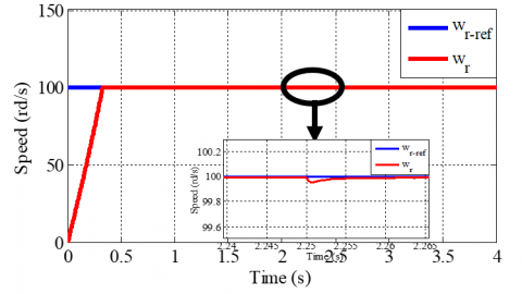
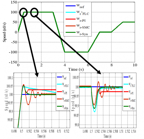
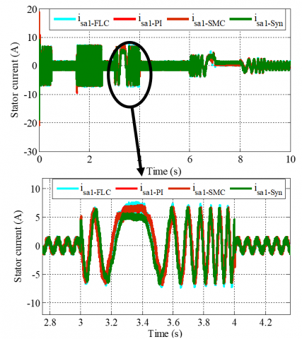
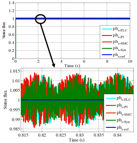
Figure 8 shows the performance of each controller when the chosen form of reference speed is a stair curve. It noticed that the synergetic controller has the best performances in following of wire speed (Figure 8(a)), the wire speed achieves its reference value quickly which prove the rapid convergence and the shirt time response of the proposed approach, the electromagnetic torque and the stator current track the chosen variation of wire speed (Figures 8(b), 8(c)), despite these changes the stator flux follows its reference value perfectly (Figure 8(d)).
(a)
(b)
(c)
(d)
Figure 8. Speed, torque, stator current and flux responses for the reference tracking test
6.2.2 Robustness test
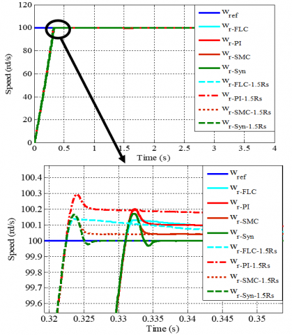
To study the robustness of the used approach, the value of the stator and rotor resistance Rs and Rr are increased by 50%, simulation results are illustrated in Figures 9-10.
(a)
(b)
(c)
(d)
Figure 9. Speed, torque, stator current and flux responses for the robustness test (an increase of stator resistance by 50%)
(a)
(b)
(c)
(d)
Figure 10. Speed, torque, stator current and flux responses for the robustness test (an increase of rotor resistance by 50%)
Figures 9-10 shows that the rotor speed, torque, stator current and flux have a clear effect due to the rotor and stator resistance variations and the effect appears more important to FLC, PI and SMC control scheme compared to a synergetic approach. It noticed also that the overshoots and the undershoots are minimized with synergetic control compared to other controllers.
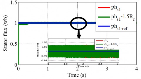
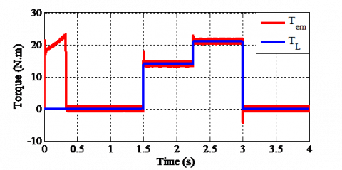
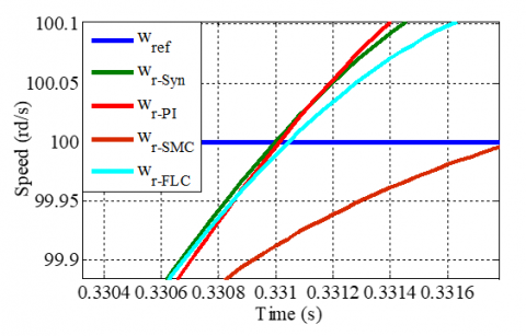
The Figure 11, the Figure 12 and the Figure 13 show the zoom in the torque, the stator flux and the speed responses respectively, Table 2 summarize the main current THD and Table 3 illustrate the amplitude of ripples for each controller.
These results show that the use of synergetic has led us to the reduced ripple amplitude and THD current, in addition to an improvement in rise time.
Table 2. SC, SMC, PI and FLC corresponding phase current THD
|
|
SC |
SMC |
PI |
FLC |
|
Current THD % |
5.85% |
6.29% |
6.1% |
6.34% |
Figure 11. Zoom in the torque response
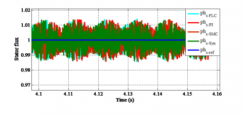
Figure 12. Zoom in the stator flux response
Figure 13. Zoom in the speed response
Table 3. Amplitude of ripples
|
|
SC |
SMC |
PI |
FLC |
|
Torque |
13.65-14.4 |
13.35-14.66 |
13.48-14.86 |
12.96-15.22 |
|
ripples (N.m) |
(0.75) |
(1.31) |
(1.38) |
(2.26) |
|
Stator |
0.9947-1.002 |
0.9898-1.009 |
0.9861-1.006 |
0.9874-1.011 |
|
Flux ripples (Wb) |
(0.0073) |
(0.0192) |
(0.0199) |
(0.0236) |
A new approach for the DTC scheme of DSIM based on synergetic control theory (SCT) was investigated in this paper. Application of the SCT allowed us to design analytical control strategy using a nonlinear model of DSIM that regulates the speed and flux continuously. These controllers guarantee asymptotic stability of the closed loop system through Lyapunov’s theory. In the first part of simulation, the performances of the used approach have been tracked and evaluated. In the second part of simulation, the controllers were assessed and compared with the classic PI, Sliding Mode (SM) and Fuzzy Logic (FL) controllers considering state and transients behaviors in DSIM. From the simulation results, it was observed that the controllers based on SCT showed better performance in all cases considered compared to the classic PI, SM and FL controllers such as: variation DSIM parameter, overload torque, THD stator current, stator flux and electromagnetic torque ripples.
|
DTC |
Direct Torque Control |
|
DSIM |
Double Star Induction Motor |
|
PI |
Proportional-Integral |
|
SMC |
Sliding Mode Control |
|
FLC |
Fuzzy Logic Control |
|
SCT |
Synergetic Control Theory |
|
Vds1,2, Vqs1,2 |
d, q axis stator voltage |
|
Vdr, Vqr |
d, q axis rotor voltage |
|
ids1,2, iqs1,2 |
d, q axis stator current |
|
idr, iqr |
d, q axis rotor current |
|
Rs1,2 |
Stator resistance |
|
Rr |
Rotor resistance |
|
v(a, b,c)s1,2 |
Stator voltage |
|
i(a, b, c)s1.2 |
Stator current |
|
(a; b, c)s1,2 |
Stator flux |
|
v(a, b, c)r |
Rotor voltage |
|
i(a, b, c)r |
Rotor current |
|
ϕ(a, b, c)r |
Rotor flux |
|
Ls1,2 |
Stator inductance |
|
Lr |
Rotor inductance |
|
Lm |
Mutual inductance |
|
ωr |
Rotor speed |
|
ωs |
Synchronism speed |
|
Tem |
Electromagnetic torque |
|
J |
Inertia moment |
|
TL |
Load torque |
|
Kf |
Friction factor |
|
X |
State system |
|
u |
Vector control |
|
T |
Control parameter |
|
P |
Poles pair number |
|
Greek symbols |
|
|
α, β |
Control parameters |
|
ϕds1,2, ϕqs1,2 |
d, q axis stator flux |
|
ϕdr, ϕqr |
d, q axis rotor flux |
|
ϕas1,2, ϕbs1,2 |
a, b axis stator flux |
|
$\Psi$ |
Macro variable |
|
ψ |
Function chosen by the user |
[1] Kortas, I., Sakly, A., Mimouni, M.F. (2017). Optimal vector control to a double-star induction motor. Energy, 131: 279-288. http://dx.doi.org/10.1016/j.energy.2017.03.058
[2] Hammache, H., Moussaoui, D., Marouani, K., Hamdouche, T. (2008). Magnetic properties in double star induction machine. 18th International Conference on Electrical Machines, pp. 1-6. http://dx.doi.org/10.1109/ICELMACH.2008.4799961
[3] Azib, A., Ziane, D., Rekioua, T., Tounzi, A. (2016). Robustness of the direct torque control of double star induction motor in fault condition. Revue Roumaine des Sciences Techniques - Serie Électrotechnique et Énergétique, 61(2): 147-152.
[4] Hamidia, F., Abbadi, A., Boucherit, M.S. (2015). Direct torque controlled dual star induction Motors (in open and closed loop). In 2015 4th International Conference on Electrical Engineering (ICEE) IEEE, pp. 1-6. https://doi.org/10.1109/INTEE.2015.7416772
[5] Youb, L., Belkacem, S., Naceri, F., Cernat, M., Pesquer, L.G. (2018). Design of an adaptive fuzzy control system for dual star induction motor drives. Advances in Electrical and Computer Engineering, 18(3): 37-44. https://doi.org/10.4316/AECE.2018.03006
[6] Lazreg, M.H., Bentaallah, A. (2019). Sensorless speed control of double star induction machine with five level DTC exploiting neural network and extended Kalman filter. Iranian Journal of Electrical and Electronic Engineering, 15(1): 142-150. https://doi.org/10.22068/IJEEE.15.1.142
[7] Zheng, L., Fletcher, J.E., Williams, B.W., He, X. (2010). A novel direct torque control scheme for a sensorless five-phase induction motor drive. IEEE Transactions on Industrial Electronics, 58(2): 503-513. https://doi.org/10.1109/TIE.2010.2047830
[8] Vasudevan, M., Arumugam, R., Paramasivam, S. (2006). Development of torque and flux ripple minimization algorithm for direct torque control of induction motor drive. Electrical Engineering, 89(1): 41-51. http://dx.doi.org/10.1007/s00202-005-0319-x.
[9] Gowri, K.S., Reddy, T.B., Babu, C.S. (2010). Direct torque control of induction motor based on advanced discontinuous PWM algorithm for reduced current ripple. Electrical Engineering, 92(7-8): 245-255. https://doi.org/10.1007/s00202-010-0182-2
[10] Araria, R., Berkani, A., Negadi, K., Marignetti, F., Boudiaf, M. (2020). Performance analysis of DC-DC converter and DTC based fuzzy logic control for power management in electric vehicle application. Journal Européen des Systèmes Automatisés, 53(1): 1-9. http://doi.org/10.18280/jesa.530101
[11] Boukhalfa, G., Belkacem, S., Chikhi, A., Benaggoune, S. (2018). Direct torque control of dual star induction motor using a fuzzy-PSO hybrid approach. Applied Computing and Informatics. http://dx.doi.org/10.1016/j.aci.2018.09.001
[12] Yue, Y.T., Lin, Y. (2015). A novel sensorless fuzzy sliding-mode control of induction motor. International Journal of Control and Automation, 8(9): 1-10. https://doi.org/10.14257/ijca.2015.8.9.01
[13] Hamouda, N., Babes, B., Hamouda, C., Kahla, S., Ellinger, T., Petzoldt, J. (2020). Optimal tuning of fractional order proportional-integral-derivative controller for wire feeder system using ant colony optimization optimal tuning of fractional order proportional-integral-derivative controller for wire feeder system using ant colony optimization. Journal Européen des Systèmes Automatisés, 53(2): 157-166. http://doi.org/10.18280/jesa.530201
[14] Amimeur, H., Aouzellag, D., Abdessemed, R., Ghedamsi, K. (2012). Sliding mode control of a dual-stator induction generator for wind energy conversion systems. International Journal of Electrical Power & Energy Systems, 42(1): 60-70 http://dx.doi.org/10.1016/j.ijepes.2012.03.024
[15] Cherifi, D., Miloud, Y. (2020). Hybrid control using adaptive fuzzy sliding mode control of doubly fed induction generator for wind energy conversion system. Periodica Polytechnica Electrical Engineering and Computer Science, 64(4): 374-381. http://dx.doi.org/10.3311/PPee.15508
[16] Rahali, H., Zeghlache, S., Benyettou, L., Benalia, L. (2019). Backstepping sliding mode controller improved with interval type-2 fuzzy logic applied to the dual star induction motor. International Journal of Computational Intelligence and Applications, 18(02): 1950012. https://doi.org/10.1142/S1469026819500123
[17] Yu, X., Jiang, Z., Zhang, Y. (2008). A synergetic control approach to grid-connected, wind-turbine doubly-fed induction generators. In 2008 IEEE Power Electronics Specialists Conference IEEE, pp. 2070-2076. https://doi.org/10.1109/PESC.2008.4592248
[18] Hossine, G., Katia, K. (2017). Improvement of vector control of dual star induction drive using synergetic approach. In 2017 14th International Multi-Conference on Systems, Signals & Devices (SSD), IEEE, pp. 643-648. http://dx.doi.org/10.1109/SSD.2017.8167006
[19] Takahashi, I., Noguchi, T. (1986). A new quick-response and high-efficiency control strategy of an induction motor. IEEE Transactions on Industry Applications, 5: 820-827. http://dx.doi.org/10.1109/TIA.1986.4504799
[20] Son, Y.D., Heo, T.W., Santi, E., Monti A. (2004). Synergetic control approach for induction motor speed control. In 30th Annual Conference of IEEE Industrial Electronics Society, 2004. IECON 2004, 1: 883-887. http://dx.doi.org/10.1109/IECON.2004.1433432
[21] Medjbeur, L., Harmas, M.N., Benaggoune, S. (2012). Robust induction motor control using adaptive fuzzy synergetic control. Journal of Electrical Engineering, 12(1): 37-42.
[22] Nusawardhana, Zak, S.H., Crossley, W.A. (2007). Nonlinear synergetic optimal controllers. Journal of Guidance, Control, and Dynamics, 30(4): 1134-1147. https://doi.org/10.2514/1.27829
[23] Davoudi, A., Bazzi, A.M., Chapman, P.L. (2008). Application of synergetic control theory to nonsinusoidal PMSMs via multiple reference frame theory. In: 2008 34th Annual Conference of IEEE Industrial Electronics, IEEE, pp. 2794–2799. https://doi.org/10.1109/IECON.2008.4758401