Haoying Fan* | Daobing Liu | Liugen Li | Guoxiao Liu
© 2020 IIETA. This article is published by IIETA and is licensed under the CC BY 4.0 license (http://creativecommons.org/licenses/by/4.0/).
OPEN ACCESS
The purpose of this study was to investigate a simplified distributed generation (DG) Position and Capacity Determination model (DG-PCD model) based on the coupling relationship between load distribution and voltage stability in the distribution network. First, based on the relationship between voltage stability and system equivalent impedance and the relationship between system equivalent impedance and load distribution, the relationship between voltage stability and load distribution is deduced, and the concept of influencing impedance mode is proposed and used in DG site selection. Then, build a DG-PCD model considering voltage stability, active power loss and line thermal stability margin, and use genetic algorithm (GA) to solve the model. Finally, an improved IEEE33-node system calculation example is analyzed. The results show that compared with the existing methods, the proposed method can get better results faster. This Proposed method not only simplifies the DG-PCD model, but also quantifies the relationship between voltage stability and load distribution. This provides a new reference index for the voltage control of the power grid.
voltage stability, load distribution, Distributed Generation (DG), influence impedance mode, position and capacity determination
As the concept of green development has entered and implemented in the field of electricity generation, DG has occupied an increasing proportion in electricity networks, and the research focus of domestic and foreign academic circles has shifted from centralized power generation to distributed power generation [1]. Due to the characteristics of DG [2, 3], unreasonable DG access schemes not only waste resources, but also lower system operation security [4, 5]. Therefore, reasonably and effectively considering the problem of DG position and capacity determination is of great significance to the safe operation of distribution networks.
Regarding DG position and capacity determination, domestic and foreign scholars have obtained a few research results. For example, Hung et al. [6] proposed three different analysis expressions to determine the optimal DG capacity and operation strategy under the condition of minimum loss, and gave the method of optimal position determination. Naik et al. [7] took the minimum network system loss as the objective function and solved the constructed model using an improved optimization algorithm. Moradi et al. [8] established a planning model with minimum network loss, minimum voltage offset, and minimum short-circuit current as objective functions. Borges and Falcao [9] analyzed the relationship between the radiation network and the DG and proposed an optimal configuration method for connecting a single DG to the radiation network. Wang and Zheng [10] considers the influence of different types of DG on the DG planning model. Mokgonyana et al. [11] further optimizes the economy after DG is connected by subdividing DG output characteristics. Tu et al. [12] simulates the uncertainty of DG output through data, and uses an extreme learning machine to solve the model. Acharya et al. [13] analyzed the sensitivity of nodes to the active power network loss of the system and took it as the basis for DG position selection; however, the robustness of this method was not satisfactory. Pham et al. [14] proposed a new intelligent algorithm to solve existing models, which has faster convergence than existing algorithms.
The existing research papers seldom consider the voltage issue. Wu et al. [15] verifies the influence of DG location and capacity on the voltage level of the distribution network from the perspective of DG access location, capacity and network loss. Shao et al. [16] analyzes the influence of DG penetration rate on power loss, reliability and voltage distribution of the grid. Moradi and Abedini [17] established a model based on typical medium voltage distribution network to study the problem of DG access capacity and position from the aspects of reverse power and voltage. Moradi and Abedini [18] used GA and particle swarm optimization (PSO) to solve the problem of DG access capacity and position, so as to minimize the system network loss, better regulate the voltage, and improve voltage stability. Prakash and Khatod [19] used loss formula and voltage sensitivity coefficient to determine the position and capacity of DG in the distribution network, which effectively reduced the network loss of the system and improved the voltage quality. Hu et al. [20] explored the maximum penetration rate of DG when the static voltage stability of the grid reaches the limit. Existing studies hadn’t taken into consideration the coupling relationship between load distribution and voltage stability, but taken DG access position and capacity as decision variables to construct and solve mathematical planning models with voltage stability as the objective. However, due to the large number of nodes in the distribution network and the large calculation dimension, the convergence effects can hardly be guaranteed.
Aiming at the shortcomings of existing research, this paper started with an analysis of the relationship between load distribution and voltage stability, and proposed a scheme of DG position and capacity determination with load distribution taken into account. First, the coupling relationship between the static voltage stability and the equivalent impedance of the node system was derived from the Thevenin equivalent circuit of the node system. Then, the relationship between the system load distribution and the node system equivalent impedance was obtained based on the superposition theorem; and the influence impedance mode, an evaluation index reflecting the impact of loads on voltage stability, was proposed and applied to DG position selection with the access capacity of DG as the decision variable. The proposed scheme can effectively reduce the calculation dimension of the model and improve the convergence effects.
In a power system, when the load accessed to the system exceeds the system limit, the voltage will drop uncontrollably and the system voltage will collapse. Most of the existing literatures took static voltage stability as the index to characterize the voltage stability of the system. Liu et al. [21] derived the static voltage stability index of the distribution network from the branch current iteration formula, as follows:
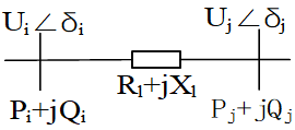
Figure 1 show the model of the branches of a distribution network, in the figure, i is the head node; j is the tail node; Ui$\angle$δi and Uj$\angle$δj respectively represent the voltages of the two nodes; Pi+Qi and Pj+Qj are the output power values of the two nodes; the impedance of branch l is Rl+Xl.
Figure 1. Distribution network branch model
The complex power equation of node j is:
$\mathrm{P}_{\mathrm{j}}+\mathrm{jQ}_{\mathrm{j}}=\dot{\mathrm{U}}_{\mathrm{j}} * \mathrm{I}_{\mathrm{j}}^{*}$ (1)
The VCR equation of the impedor is:
$\overset{\bullet }{\mathop{{{\text{I}}_{j}}}}\,=\frac{{{\overset{\bullet }{\mathop{U}}\,}_{i}}-{{\overset{\bullet }{\mathop{U}}\,}_{j}}}{{{R}_{l}}+j{{X}_{l}}}$ (2)
Combine Eqns. (1) and (2) to get the network equation as:
$\begin{align} & \text{U}_{\text{j}}^{\text{4}}+(2{{P}_{j}}{{R}_{l}}+2{{Q}_{j}}{{X}_{l}}-U_{i}^{2})\text{U}_{\text{j}}^{\text{2}}+(R_{l}^{2}+ \\ & X_{l}^{2})(P_{j}^{2}+Q_{j}^{2})=0 \\ \end{align}$ (3)
Based on the solvability of the equation, define the node voltage stability margin index as:
${{\text{L}}_{j}}=\frac{4}{U_{i}^{4}}[{{({{P}_{j}}{{X}_{l}}-{{Q}_{j}}{{R}_{l}})}^{2}}+({{P}_{j}}{{R}_{l}}+{{Q}_{j}}{{X}_{l}})U_{i}^{2}]$ (4)
According to Eq. (4), when Lj <1, the node voltage is in a stable state; when Lj=1, the node voltage is in a critical stable state; when Lj>1, the node voltage is unstable. Under the condition of an L value less than 1, the smaller the L value, the more stable the node voltage.
In a distribution network with n nodes, the system voltage stability index L is defined as:
$\text{L}=\underset{j\in [1,n]}{\mathop{\max }}\,({{L}_{j}})$ (5)
It is the value of the static voltage stability index of the weak nodes in the system; this is because the system collapse always starts from the weakest branch in the system.
Essentially, the static voltage stability index evaluates the gap between the current operating state and the limit state. When there’s not much changes in the current operating state, increasing the limit load [22] of the nodes can effectively improve their static voltage stability.
In a multi-node system, when the network structure is determined, the equivalent impedance of the node system depends on the distribution mode of system load. In order to characterize this coupling relationship scientifically and reasonably, this paper derived a concept of influence impedance mode considering the coupling relationship between load distribution and node voltage.
3.1 The relationship between voltage stability and system equivalent impedance
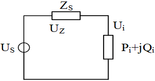
Figure 2 is the Thevenin equivalent circuit of node i, at this time, the system equivalent voltage is:
$\overset{.}{\mathop{{{\text{U}}_{s}}}}\,={{\overset{.}{\mathop{U}}\,}_{i}}+\frac{{{P}_{i}}-j{{Q}_{i}}}{{{\overset{.}{\mathop{U}}\,}_{i}}}{{Z}_{s}}$ (6)
Substitute Formula (6) into Formula (4), and differentiate ZS to obtain:
$\frac{\partial \text{L}}{\partial {{Z}_{s}}}=\frac{4U_{i}^{2}N}{{{M}^{7}}}[2U_{i}^{2}{{\text{Z}}_{\text{s}}}{{({{P}_{i}}\sin \theta -Q\cos \theta )}^{2}}-(P\text{cos}\theta +Q\sin \theta ){{M}^{3}}]$ (7)
where, $M=\left(U_{i}^{2}+P_{i} Z_{s}\right)^{2}+Q_{i}^{2} Z_{s}^{2}$, $N=U_{i}^{4}-\left(P_{i}^{2}+Q_{i}^{2}\right) Z_{S}^{2}$, θ is the impedance angle of ZS.
The range of node load under the impedance angle and the per-unit value in the distribution network is:
$\left\{\begin{array}{l}\theta \in\left[0, \frac{\pi}{2}\right] \\ P_{i}, Q_{i}, U_{i} \in[0,1]\end{array}\right.$
It can be obtained that before node i reaches the stability limit, the values of each term in Formula (7) are:
$\left\{ \begin{align} & \frac{4U_{i}^{2}}{{{M}^{7}}}>0 \\ & \\ & N=U_{i}^{2}\frac{N}{U_{i}^{2}}=U_{i}^{2}[U_{i}^{2}\text{-}\frac{(P_{i}^{2}+Q_{i}^{2})}{U_{i}^{2}}Z_{_{S}}^{2}]=U_{i}^{2}(U_{i}^{2}-U_{z}^{2})>0 \\ & \\ & \\ & 1>({{P}_{\text{i}}}\text{cos}\theta +{{Q}_{i}}\sin \theta )>2U_{i}^{2}{{({{P}_{i}}\sin \theta -Q\cos \theta )}^{2}}>0 \\ \end{align} \right.$ (8)
Formula (7) is less than 0, that is, the L value of node i decreases as Zs decreases, indicating that the size of the equivalent impedance of the node system has an impact on the static voltage stability of the node.
Figure 2. Thevenin equivalent of the system
3.2 Relationship between system equivalent impedance and load distribution
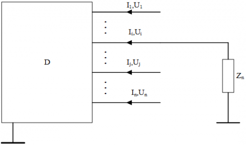
As shown in Figure 3, in a linear distribution network with n nodes, the voltage of the i-th node can be expressed as:
${{\text{U}}_{i}}=\sum\limits_{i=1}^{n}{{{Z}_{ij}}}{{I}_{j}}=\sum\limits_{i=1,i\ne j}^{n}{{{Z}_{ij}}\frac{{{\text{I}}_{j}}}{{{I}_{i}}}}+{{Z}_{ii}}$ (9)
where, Zii is the self-impedance of port i; and Zij is the mutual impedance of ports i and j. The system equivalent impedance DZi(s) of node i and the influence impedance DZij of node j on node i are defined as:
$\left\{ \begin{align} & \Delta {{\text{Z}}_{i(s)}}=\frac{{{U}_{i}}}{{{I}_{i}}}=\sum\limits_{i=1,i\ne j}^{n}{{{Z}_{ij}}\frac{{{I}_{j}}}{{{\text{I}}_{i}}}}+{{\text{Z}}_{ii}} \\ & \\ & \\ & \Delta {{\text{Z}}_{ij}}={{Z}_{ij}}\frac{{{I}_{j}}}{{{I}_{i}}}=-{{Z}_{ij}}\frac{({{P}_{j}}-j{{Q}_{j}})\overset{*}{\mathop{{{U}_{i}}}}\,}{\overset{*}{\mathop{{{U}_{j}}}}\,({{P}_{i}}-j{{Q}_{i}})} \\ \end{align} \right.$ (10)
where, P1/Q1, P2/Q2 are respectively the active/reactive loads of node 1 and node 2, obviously there is:
$\Delta {{\text{Z}}_{i(s)}}=\sum\limits_{i=1,i\ne j}^{n}{\Delta {{Z}_{ij}}+{{Z}_{ii}}}$ (11)
Before the system reaches the limit, the voltage amplitude of the distribution network does not change much, therefore, it is assumed that the voltage amplitude of the distribution network remains unchanged. At this time, according to Formulas (10) and (11), the smaller the system load, the greater the sum of the influence impedance modes of node i, and the greater the system equivalent impedance of node i, the smaller the L value of the node, and the more stable the voltage. That is, the smaller the system load, the more stable the system voltage, which conforms to reality.
Connecting DG to the distribution network will change the system load distribution and affect the voltage stability of the distribution network. However, due to the different DG access positions and capacities, the system voltage stability would be different after DG has been connected to the network. According to Formula (11), under a same DG penetration level, the greater the ΔZij value of access node, the greater the system equivalent impedance of the target node. According to Formula (7), the smaller the L value of the objective function, the more stable the system voltage. In summary, the greater the ΔZij value of the access node, the more stable the system static voltage. Therefore, the appropriate DG access position can be selected according to the influence impedance mode index.
Figure 3. Node equivalent impedance
4.1 Objective function
This paper established a multi-objective DG-PCD model with active power network loss, static voltage stability of system and thermal stability margin of circuits as sub-objective functions, then the weighting method was adopted to transform it into single sub-objective functions.
4.1.1 System static voltage stability index
Reasonable DG access can improve the system voltage stability. In this paper, the minimum system static voltage stability index had been taken as a sub-objective function, namely:
f1=min(L) (12)
4.1.2 Active power network loss index
Connecting DG to the power grid can reduce branch power flow, namely the branch network loss. However, excessive DG capacity may cause the power flow of the power grid to flow in the reverse direction, which will increase the branch network loss. The active power network loss was taken as a sub-objective function, that is:
$\text{min}{{\text{f}}_{\text{2}}}={{\text{P}}_{loss}}=\underset{l=1}{\overset{N}{\mathop{\Sigma }}}\,{{P}_{l}}$ (13)
where, Pl is the active power loss of the branch; N is the total number of power grid branches.
4.1.3 Circuit current index
After the DG is connected to the power grid, the current on some branches may increase, causing the current of some circuits to exceed the limit and thus affecting the normal operation of the system. Define Imax as the maximum value of the system branch current, namely the thermal stability current of the circuit:
${{\text{I}}_{\max }}=\underset{i=1}{\overset{N}{\mathop{\max }}}\,({{I}_{l}})$ (14)
The minimum thermal stability margin of the circuit was taken as a sub-objective function to improve the thermal stability of the system circuit, that is:
f3=min(Imax) (15)
4.2 Constraints
(1) Power balance constraint:
$\left\{\begin{array}{l}P_{s}+\sum_{i \in[1, n]}^{n} P_{D G i}=P_{\text {Load}}+P_{\text {Loss}} \\ Q_{s}+\sum_{i \in[1, n]}^{n} Q_{D G i}=Q_{\text {Load}}+Q_{\text {Loss}}\end{array}\right.$ (16)
where, Ps and Qs are respectively the active power and the reactive power delivered by the upper-level grid when the DG is not connected to the grid; PDGi and QDGi are the active/reactive power of each node when DG is connected; PLoad and QLoad are the active/reactive power of the distribution network; Ploss and Qloss are the active power network loss and reactive power network loss of the system.
(2) Voltage constraint
In order to ensure the safe and stable operation of the power system, the voltage of each node must be kept within a specified range, namely:
${{\text{U}}_{i\min }}\le \underset{i\in [1,n]}{\mathop{{{U}_{i}}}}\,\le {{U}_{i\max }}$ (17)
(3) DG access capacity constraint
According to Lu et al. [23], excessive DG capacity will lower the voltage stability of the system, therefore, this paper set that the penetration rate of DG did not exceed 30%:
$\left\{\begin{array}{l}\sum_{i \in[1, n]}^{n} P_{D G i} \leq 30 \% \times P_{L o a d} \\ \sum_{i \in[1, n]}^{n} Q_{D G i} \leq 30 \% \times Q_{L o a d}\end{array}\right.$ (18)
4.3 Non-dimensionalization and weighting
Since each sub-objective function had a different dimension, the range normalization method in reference [24] was adopted to make each of them dimensionless, the method is:
$y_{i j}=\frac{x_{i j}-\min \left\{x_{i j}\right\}}{\max _{i}\left\{x_{i j}\right\}-\min _{i}\left\{x_{i j}\right\}}$ (i=1,2,..,m;j=1,2,..,n) (19)
where, xij represents the actual value of index j of evaluation scheme i. Max{xij}/Min{xij} are the maximum/minimum values of xij. yij is the value of the evaluation index after range normalization, yij $\in$[0,1].
Then the weighting method was adopted to normalize the multi-objective function into single objective functions, namely:
$\text{f}={{w}_{1}}f_{1}^{*}+{{w}_{2}}f_{2}^{*}+{{w}_{3}}f_{_{3}}^{*}$ (20)
where, wi is the weight coefficient, and f3* is the dimensionless objective function.
5.1 Parameter setting
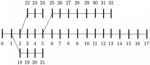
This paper used an improved GA to simulate an IEEE 33-node system in Matlab. The topology of the 33-node system is shown in Figure 4, which has 32 branches, the system reference voltage UB=12.66kV, and the reference power SB=10MW; see Appendix A for the loads of each node and the branch circuit parameters. In the calculation example, two DGs had been installed in the system. Considering the actual engineering requirements, the DG capacity was set to be an integer multiple of 10, the total capacity installed did not exceed 30% of the total load of the system; and the DG power factor was set to 0.9. Considering the system voltage stability and the circuit thermal stability, this paper set the upper and lower limits of node voltage fluctuations to 5%, and the maximum circuit current was not allowed to exceed 500A.
Figure 4. Topology of a 33-node system
The parameters of the improved GA [25] were: initial population n=100; chromosome length 33; the maximum iterations Genmax=150; crossover factor Pcro=0.5; mutation factor Pmut=0.1. According to the data in Literature [24], the objective function weights were set as w1=0.4286, w2=0.4286, and w3=0.1428.
5.2 Analysis of the example
First, the influence impedance mode was adopted to quantify the coupling relationship between the nodes. Taking root node 0 as the reference node, the system node impedance matrix was obtained. Then, according to the power flow distribution of the initial load, the influence impedance mode between each node was solved, and the results are shown in Figure 5.
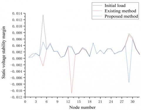
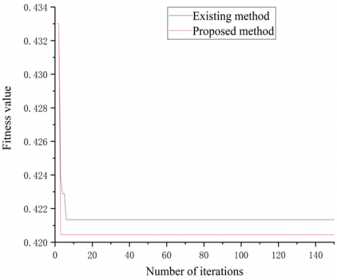
It can be seen from Figure 6 that under the initial load, the voltage stability margin index of Node 5 was 0.0133, which was much greater than other nodes; therefore, it was the weak node of the system. According to Figure 5, the two nodes with the largest influence impedance with Node 5 were Node 29 and Node 5, so they were selected as the DG access positions. Then the DG-PCD model was solved based on the above-mentioned parameters and compared with an existing method (DG access position and capacity were taken as decision variables of the model, solved by the same GA), the results are shown in Figure 7. The traditional method generally takes the DG access position as the decision variable, which would result in that the computation amount of the model increases geometrically, and it’s easy to fall into the local optimal solution. Since the quantification of DG access position determination process reduces the computation amount, the proposed model has faster convergence speed and better solutions.
Figure 5. Influence impedance modes between nodes
Figure 6. Values of node static voltage stability index for different DG installation schemes
Under the initial load, the power flow can be calculated by the forward-back substitution, the system active power network loss was 197.3760kW, the maximum static voltage stability index was 0.0133, appeared at node 5. According to Figure 6, after DG was connected, the system static voltage stability index had been greatly reduced, and the system voltage stability had been improved. The proposed method showed faster convergence speed and obtained better results, which had proved that, by reducing the calculation dimension, the solution speed had been improved. The proposed method had found a better DG access scheme than existing method. According to Figure 8, after the DG was connected, the voltage distribution in the system had been greatly improved. Compared with the existing method, the method proposed in this paper better improved the voltage distribution.
Figure 7. Comparison of convergence of each method
Figure 8. Per-unit values of node voltage for different DG installation schemes
Table 1. DG installation schemes
|
Scheme |
DG access position |
DG access capacity/kw |
Influence impedance mode |
System voltage stability margin (×10-3) |
Network loss/KW |
Maximum branch current amplitude /A |
Comprehensive objective function value |
|
1 |
- |
- |
- |
133 |
197.3760 |
463.9000 |
0.8903 |
|
2 |
5 |
290 |
0.1649 |
58 |
84.8871 |
327.6500 |
0.4199 |
|
29 |
940 |
0.2227 |
|||||
|
3 |
5 |
570 |
0.1649 |
72 |
92.7513 |
325.8500 |
0.4806 |
|
13 |
660 |
0.0509 |
|||||
|
4 |
5 |
320 |
0.1649 |
72 |
99.9473 |
327.7000 |
0.4929 |
|
8 |
910 |
0.0219 |
|||||
|
5 |
7 |
350 |
0.0770 |
130 |
81.3919 |
327.1500 |
0.6470 |
|
29 |
880 |
0.2227 |
Table 1 shows the comparison results of the function indexes of different DG installation schemes, wherein Scheme 1 shows the target values of the system under the condition of no DG access; Scheme 2 is the solution of the proposed method; and Scheme 3 is the solution of the existing method. After DG had been connected to the power grid, the various indexes of the system had obvious improvements. In Scheme 2, since the influence impedance mode of node 29 was greater than that of node 5, therefore the DG access capacity of node 29 was also greater than that of node 5, which indicated that the proposed method is reasonable. Moreover, the comparison between Scheme 2 and Scheme 3 also showed the superiority of the proposed method in all aspects. Although the values of the total objective function and sub-objective functions of Scheme 4 were slightly worse than Scheme 3, in terms of sub-objectives and total objective, it was not as good as Scheme 2. Scheme 5 had the least network loss, but in terms of the values of other sub-objective functions and the total objective function, it was much greater than Scheme 2. In conclusion, Scheme 2 should be adopted.
This paper proposed a planning scheme for DG access position and capacity in distribution networks. The scheme took the influence of load distribution into account and separated position determination and capacity determination, then a multi-objective model considering the system static voltage stability, active power network loss and circuit thermal stability margin was established, and an improved GA was applied to solve the model. The research conclusions are:
1) The paper deduced the change trends of node voltage stability and system equivalent impedance, and proposed the concept of influence impedance mode based on the coupling relationship between load distribution and system equivalent impedance. Then, through the influence impedance mode, the problems of DG position and capacity determination were separated, the computation dimension of the model was reduced, and the computation speed was improved.
2) The proposed method not only can effectively simplify the DG-PCD model, but also offered a reference for assessing the system's static voltage stability. However, the proposed method was not able to quantify the coupling relationship between load distribution and system static voltage stability.
3) In subsequent research, we plan to explore the relationship between the maximum DG access capacity and load distribution of each node in the system, and consider the influence of DG type on its position and capacity determination, in the hopes of providing more accurate references for actual engineering projects.
[1] Javier, B., Hector, C., Karina, A.B., Marcela, J., Rodrigo, A. (2020). A simple distribution energy tariff under the penetration of DG. Energies, 13(8): 1910. http://doi.org/10.3390/en13081910.
[2] Abushamah, H.A.S., Haghifam, M.R., Bolandi, T.G. (2020). A novel approach for distributed generation expansion planning considering it’s added value compared with centralized generation expansion. Sustainable Energy, Grids and Networks, 25: 100417. http://doi.org/10.1016/j.segan.2020.100417
[3] Arabi, A., Ramezani, M., Falaghi, H. (2016). Probabilistic evaluation of available load supply capability of distribution networks as an index for wind turbines allocation. IET Renewable Power Generation, 10(10): 1631-1637. http://doi.org/10.1049/iet-rpg.2015.0350
[4] Nguyen, T.T., Nguyen, T.T., Nguyen, N.A., Duong, T.L. (2020). A novel method based on coyote algorithm for simultaneous network reconfiguration and distribution generation placement. Ain Shams Engineering Journal, 41(8): 129-136. http://doi.org/10.1016/j.asej.2020.06.005
[5] Shradha, S.P., Nitin, M. (2020). Optimal allocation of renewable DGs in a radial distribution system based on new voltage stability index. International Transactions on Electrical Energy Systems, 30(4): e12295. http://doi.org/10.1002/2050-7038.12295
[6] Hung, D.Q., Mithulananthan, N., Bansal, R.C. (2013). Analytical strategies for renewable distributed generation integration considering energy loss minimization. Applied Energy, 105(2): 75-85. http://doi.org/10.1016/j.apenergy.2012.12.023
[7] Naik, S.G., Khatod, D.K., Sharma, M.P. (2013). Optimal allocation of combined DG and capacitor for real power loss minimization in distribution networks. International Journal of Electrical Power & Energy Systems, 53: 967-973. http://doi.org/10.1016/j.ijepes.2013.06.008
[8] Moradi, M.H., Tousi, S.R., Abedini, M. (2014). Multi-objective PFDE algorithm for solving the optimal siting and sizing problem of multiple DG sources. International Journal of Electrical Power & Energy Systems, 56: 117-126. http://doi.org/10.1016/j.ijepes.2013.11.014
[9] Borges, C.L., Falcao, D.M. (2006). Optimal distributed generation allocation for reliability, losses, and voltage improvement. International Journal of Electrical Power & Energy Systems, 28(6): 413-420. http://doi.org/10.1016/j.ijepes.2006.02.003
[10] Wang, Y.N., Zheng, T. (2019). Site selection and capacity determination of multi-types of DG in distribution network planning. In IOP Conference Series: Materials Science and Engineering, 486(1): 012071. http://doi.org/10.1088/1757-899X/486/1/012071
[11] Mokgonyana, L., Zhang, J., Li, H., Hu, Y. (2017). Optimal location and capacity planning for distributed generation with independent power production and self-generation. Applied Energy, 188: 140-150. http://doi.org/10.1016/j.apenergy.2016.11.125
[12] Tu, J., Xu, Y., Yin, Z. (2019). Data-driven kernel extreme learning machine method for the location and capacity planning of distributed generation. Energies, 12(1): 109. http://doi.org/10.3390/en12010109
[13] Acharya, N., Mahat, P., Mithulananthan, N. (2006). An analytical approach for DG allocation in primary distribution network. International Journal of Electrical Power & Energy Systems, 28(10): 669-678. http://doi.org/10.1016/j.ijepes.2006.02.013
[14] Pham, T.D., Nguyen, T.T., Dinh, B.H. (2020). Find optimal capacity and location of distributed generation units in radial distribution networks by using enhanced coyote optimization algorithm. Neural Computing and Applications, pp. 1-29. http://doi.org/10.1007/s00521-020-05239-1
[15] Wu, W., Guo, N., Deng, Z., Yu, H., Hu, G., Zhu, B., Zhao, H. (2019). Analysis of influence of distributed power supply on distribution network voltage considering permeability. E&ES, 227(3): 032039. http://doi.org/10.1088/1755-1315/227/3/032039
[16] Shao, H., Shi, Y., Yuan, J., An, J., Yang, J. (2018). Analysis on voltage profile of distribution network with distributed generation. In IOP Conf. Ser. Earth Environ. Sci. 113: 012170. http://doi.org/10.1088/1755-1315/113/1/012170
[17] Moradi, M.H., Abedini, M. (2012). A combination of genetic algorithm and particle swarm optimization for optimal distributed generation location and sizing in distribution systems with fuzzy optimal theory. International Journal of Green Energy, 9(7): 641-660. http://doi.org/10.1080/15435075.2011.625590
[18] Moradi, M.H., Abedini, M. (2012). A combination of genetic algorithm and particle swarm optimization for optimal DG location and sizing in distribution systems. International Journal of Electrical Power & Energy Systems, 34(1): 66-74. http://doi.org/10.1016/j.ijepes.2011.08.023
[19] Prakash, P., Khatod, D.K. (2016). Optimal sizing and siting techniques for distributed generation in distribution systems: A review. Renewable and Sustainable Energy Reviews, 57: 111-130. http://doi.org/10.1016/j.rser.2015.12.099
[20] Hu, L., Liu, K.Y., Sheng, W., Diao, Y., Jia, D. (2017). Research on maximum allowable capacity of distributed generation in distributed network under global energy internet considering static voltage stability. The Journal of Engineering, 2017(13): 2276-2280. http://doi.org/10.1049/joe.2017.0736
[21] Liu, J., Bi, P., Dong, H. (2002). Simplified Analysis and Optimization of Complex Distribution Network. China Electric Power Press, Beijing, China. pp. 140-144.
[22] Shi, H.L. (2010). The Generalized Thevenin Equivalence Principle of Power System Voltage Stability Analysis. Hunan University.
[23] Lu, T., Tang, W., Cong, P.W., Bo, B. (2013). Multi-objective coordinated planning of distributed power and distribution grids. Automation of Electric Power Systems, 37(21): 139-145. http://doi.org/10.7500/AEPS201301011
[24] Lu, G.H., Teng, H., Liao, H.X., Wu, Z.Q. (2019). Location selection and capacity determination of distributed power sources based on improved beetle search algorithm. Electrical Measurement and Instrumentation, 56(17): 6-12.
[25] Chai, Z.L. (2017). Research on location and capacity of distributed power generation based on improved genetic algorithm. Tianjin University.