Yanghua Gao* | Weidong Lou | Hailiang Lu | Yonghua Jia
© 2020 IIETA. This article is published by IIETA and is licensed under the CC BY 4.0 license (http://creativecommons.org/licenses/by/4.0/).
OPEN ACCESS
This paper mainly explores the consensus control of multi-agent robot system with repetitive motion under the constraints of a leader and fixed topology. To realize the consensus control, a fractional order iterative learning control (FOILC) algorithm was designed under the mode of distributed open-closed-loop proportional-derivative alpha (PDα). The uniform convergence of the algorithm in finite time was discussed, drawing on factional calculus, graph theory, and norm theory, resulting in the convergence conditions. Theoretical analysis shows that, with the growing number of iterations, each agent can choose the appropriate gain matrix, and complete the tracking task in finite time. The effectiveness of the proposed method was verified through simulation.
multi-agent robot system, fractional-order iterative learning control (FOILC), state delay, consensus control
The multi-agent robot system can complete large and complex fieldwork through communication, coordination, and cooperation. The efficiency and performance of the system are much better than those of a single robot. As a result, the multi-agent robot system has been widely used in mobile robot handling, three-dimensional (3D) printing, and welding [1, 2].
The consensus control, as a representative problem of the collaborative control of the multi-agent robot system, aims to design a suitable control algorithm to regulate the state or output of each robot in a finite time. The coordination and consensus between multiple agents have attracted much attention from the academia, yielding fruitful results [3-6]. However, most consensus control methods for multiple agents are based on integer-order descriptions of the agents, that is, the differential equations of the robots are of integer-order [7, 8].
In complex natural environments (e.g. material mechanics, motor systems, and robots), it is more accurate to describe robot dynamics with fractional calculus than integer calculus [9, 10]. Strictly speaking, the integer-order system is a special case of the fractional-order system. Therefore, many scholars engaging in multi-agent robot system have turned their attention from the integer-order model to the fractional-order model [11-14].
Yu et al. [11, 12] pioneered the study of consensus control of fractional-order multi-agent system (FOMAS), and judged the convergence of factional multiple agents with a leader. Later, Bai et al. [13] explored the consensus control of FOMAS in fixed reference states and time-varying reference states. Ma et al. [14] introduced consensus control to fractional dynamics, and developed a consensus control algorithm based on relative output measurements. By graph theory and Lyapunov method, Yu et al. [11, 12] defined the criteria for the consensus control of nonlinear FOMAS with a leader, put forward the stability theory on fractional differential systems, and derived the matrix inequalities based on the theory. Yu et al. [15] presented the necessary and sufficient conditions for the consensus control of FOMAS with leaders, and designed an observer to solve the consensus problem. Chai et al. [16] and Sun et al. [17] realized consensus control of FOMAS with adaptive control, and sliding mode control, respectively.
Most of the above studies focus on the consensus control with gradual convergence. However, the FOMAS with repetitive motions, such as the coordinated operation of multiple manipulators on a production line, generally require the control algorithm to converge within a finite time. The methods of the above research cannot satisfy this requirement.
Among the current control methods, iterative learning control can complete the tracking task in a finite time. This method has been applied to various models of integer-order multi-agent system (IOMAS) [18-20]. But there is little report on the fractional-order iterative learning control (FOILC) of FOMAS. To make matters worse, the actual FOMAS often face state delays induced by digital signal processors (DSPs), communication processors, and other processors. Hence, it is of engineering significance to solve the consensus control of FOMAS with state delay.
Considering the state delay in FOMAS, this paper proposes several methods to solve the consensus control of FOMAS composed of robots, namely, FOLIC algorithms under the mode of open-closed-loop proportional-derivative alpha (PDα), closed-loop PDα, and, open-loop PDα. Based on graph theory, norm theory, and fractional calculus, the finite-time convergence of the proposed algorithms was theoretically proved for FOMAS with state delay. Finally, the open-closed-loop PDα FOLIC algorithm was verified to be the most effective consensus control method for FOMAS with state delay through numerical simulation.
2.1 Graph theory
For a multi-agent system of $\mathrm{n}$ fractional agents, the communication links between the multiple agents constitute a network. The network can be expressed as a directed weighted graph $G=\{V, E, M\},$ where $V=\left\{v_{1}, \cdots, v_{n}\right\}$ is the set of nodes (agents), and $E \in V \times V$ is the set of edges (communication links). Let $I=\{1,2, \cdots, n\}$ be the index set of the nodes. Then, the adjacency matrix of the network can be described as $M=\left(a_{i k}\right)_{n \times n}$ where aik is the weight of the edge between node i and node k. If node i transmits information to node k, then aik>0; otherwise aik=0. It was also assumed that no node in the network commits self-connection: aii=0 for $\mathrm{i} \in \mathrm{I}$.
Let $N_{i}=\left\{k: a_{i k}>0\right\}$ be the set of neighboring nodes of node $i$ and $D=\operatorname{diag}\left\{d_{i}, \underline{i}=1, \cdots, N\right\},$ where $d_{i}=\sum_{k=1}^{N} a_{i k}$ is the sum of the elements in row i of adjacency matrix $M .$ Hence, the Laplacian matrix of graph $G$ can be obtained as $L=D-M$. For two nodes $i$ and $k,$ if a set of subscripts $\left\{k_{1}, \cdots, k_{1}\right\}$ satisfies $a_{i k_{1}}>0, a_{i k_{1}}>0, \cdots, a_{k_{l} k}>0,$ then there exists an information transmission channel between the two nodes, such that node k can receive the information from node i. Node i is globally reachable if there is a path for it to reach any other node in the graph.
Lemma 1. For an FOMAS of n autonomous individuals, if the edges forma directed weighted network, and if there is at least one globally reachable node, then the rank of the Laplacian matrix L of the directed weighted graph is N-1, with a zero eigenvalue corresponding to the eigenvector ξ0=c[1,⋯,1]T.
2.2 Fractional calculus and norm theory
The fractional calculus adopted for this research can be defined as follows:
Definition 1. In the interval [t0, t], the $\alpha$-order fractional derivatives of function f(t) can be defined as:
${}_{{{t}_{0}}}D_{t}^{-\alpha }f(t)=\frac{1}{\Gamma (\alpha )}\int_{{{t}_{0}}}^{t}{{{(t-\tau )}^{\alpha -1}}f(\tau )}d\tau $ (1)
where, $\alpha>0 ; \Gamma(\cdot)$ is gamma function $\Gamma(\alpha)=\int_{0}^{\infty} e^{-t} t^{\alpha-1} d t$.
In the interval [t0,t], the a-order fractional Riemann-Liouville and Caputo derivatives on the function f(t) can be expressed as:
${}_{{{t}_{0}}}^{RL}D_{t}^{\alpha }f(t)=\frac{{{d}^{[\alpha ]+1}}}{d{{t}^{[\alpha ]+1}}}\left[ {}_{{{t}_{0}}}D_{t}^{-([\alpha ]-\alpha +1)}f(t) \right]$ (2)
${}_{{{t}_{0}}}^{C}D_{t}^{\alpha }f(t)={}_{{{t}_{0}}}D_{t}^{-([\alpha ]-\alpha +1)}\left[ \frac{{{d}^{[\alpha ]+1}}}{d{{t}^{[\alpha ]+1}}}f(t) \right]$ (3)
where, α is any positive real number; [α] is the integer part of α.
Lemma 2. For the continuous function f(x(t), t), there exist:
$\left\{ \begin{matrix} {}_{{{t}_{0}}}^{C}D_{t}^{\alpha }x(t)=f(x(t),t) \\ x({{t}_{0}})=x(0) \\\end{matrix},0<\alpha <1 \right.$ (4)
Then, the equivalent Volterra nonlinear integral equation for the initial value problem can be expressed as:
$x(t)=x(0)+\frac{1}{\Gamma (\alpha )}\int_{{{t}_{0}}}^{t}{{{(t-\tau )}^{\alpha -1}}f(x(\tau ),\tau )}d\tau $ (5)
Let $\mathbb{R}$ be any set of real numbers, $\mathbb{C}$ be any set of complex numbers, and $\mathbb{N}$ be the set of natural numbers. For a vector $x=\left[x_{1}, x_{2}, \cdots, x_{n}\right]^{T} \in \mathbb{R}^{n},$ the $l_{p}$ norm can be represented as $|\mathrm{x}|$, with $1 \leq p \leq \infty$. In fact, when $p$ equals $1,2,$ and $\infty$, there exist $|x|_{1}=\sum_{k=1}^{n}\left|x_{k}\right|,|x|_{2}=\sqrt{x^{T} x}, \text { and }|x|_{\infty}=\max _{k=1, \cdots, n}\left|x_{k}\right|$.Then, matrix $A \in \mathbb{R}^{n \times n}|\mathrm{~A}|$ represents the matrix norm, and $\rho(A)$ characterizes the spectral radius of matrix $A$. In addition, the Kronecker product is denoted as $\otimes$, and the $m \times m$ identity $\operatorname{matrix}$ as $I_{m}$.
2.3 FOMAS model with state delay
Suppose the FOMAS with leader contains N agents, numbered as 1, 2, 3..., N. Each agent can be modeled as:
$\left\{ \begin{align} & {{D}^{\alpha }}{{x}_{i,j}}(t)=A{{x}_{i,j}}(t-\tau )+B{{u}_{i,j}}(t) \\ & {{y}_{i,j}}(t)=C{{x}_{i,j}}(t) \\\end{align} \right.$ (6)
where, $t \in[0, T]$ (if $t \in[-h, 0],$ then $x_{i, j}(\mathrm{t})=\psi(t) ; \alpha \in(0,1) ; i$ is the number of iterations; $D^{a} x_{i j}(t)$ is the $\alpha$ -order derivative of $x_{i j}(t)$ $x_{i, j}(t) \in \mathbb{R}^{m}$ is the vector of the $j$ -th agent; $u_{i, j}(t) \in \mathbb{R}^{m 1}$ and $y_{i, j}(t) \in \mathbb{R}^{m 2}$ are the input and output, respectively; $\mathrm{A}, \mathrm{B}$ and $\mathrm{C}$ are constant matrices.
Formula (6) can be written in the multi-agent vector form as
$\left\{ \begin{align} & {{D}^{\alpha }}{{x}_{i}}\left( t \right)=\left( {{I}_{N}}\otimes A \right){{x}_{i}}\left( t\text{-}\tau \right)+\left( {{I}_{N}}\otimes B \right){{u}_{i}}\left( t \right) \\ & {{y}_{i}}\left( t \right)=\left( {{I}_{N}}\otimes C \right){{x}_{i}}\left( t \right) \\ \end{align} \right.$ (7)
where, $x_{i}(t)=\left[x_{i, 1}(t)^{T}, x_{i, 2}(t)^{T}, \cdots, x_{i, N}(t)^{T}\right]^{T} \quad ; \quad u_{i}(t)=\left[u_{i, 1}^{T}(t), u_{i, 2}^{T}(t), \cdots, u_{i, N}^{T}(t)\right]^{T} \quad ; \quad y_{i}(t)=\left[y_{i, 1}^{T}(t), y_{i, 2}^{T}(t), \cdots, y_{i, N}^{T}(t)\right]^{T} \quad ; \quad \xi_{i}(t)=\left[\xi_{i, 1}(t)^{T}, \xi_{i, 2}(t)^{T}, \cdots, \xi_{i, N}(t)^{T}\right]^{T} ; \otimes$ is the Kronecker product.
Here, the desired trajectory $y_{d}(t)$ is generated by the leader in formula (6) within the time interval [0, T]. Then, the leader can be defined as:
$\left\{ \begin{align} & {{D}^{\alpha }}{{x}_{d}}(t)=A{{x}_{d}}(t-\tau )+B{{u}_{d}}(t) \\ & {{y}_{d}}(t)=C{{x}_{d}}(t) \\\end{align} \right.$ (8)
where, ud(t) is the desired input.
Due to the limitations on communication or sensors, the leader can only communicate with some of the multiple agents. Let G{V, E} be the communication network, and zero be the serial number of the leader. Then, the entire graph containing the leader can be expressed as $\bar{G}=\{0 \cup V, \bar{E}\},$ where $\bar{E}$ is the corresponding edge in the new graph. Our main task is to design an FOILC algorithm to ensure that each agent converges to the desired trajectory in the new graph $\bar{G}$.
The distributed error ξi,j(t) can be defined as:
$\begin{align} & {{\xi }_{i,j}}(t)=\sum\nolimits_{k\in {{N}_{j}}}{{{a}_{j,k}}({{y}_{i,k}}(t)-{{y}_{i,j}}(t))} \\ & +{{d}_{k}}({{y}_{d}}(t)-{{y}_{i,j}}(t)) \\\end{align}$ (9)
where, aj,k is the weight of the (j, k)-th neighborhood of the adjacency matrix M; Nj is the domain set of the j-th agent; dk is the sum of the elements in row i of the adjacency matrix. If dj=1, then the j-th agent can receive information from the leader, i.e., $(0, j) \in \bar{E}$; if dj=0, then the j-th agent cannot receive information from the leader. The error can be expressed as ei,j(t)=yd(t)-yi,j(t).
Then, the open-closed PDα FOILC can be designed as:
$\begin{align} & {{u}_{i+1,j}}(t)={{u}_{i,j}}(t)+{{\Gamma }_{P1}}{{\xi }_{i,j}}(t)+{{\Gamma }_{D1}}{{\xi }_{i,j}}^{\left( \alpha \right)}(t) \\ & \text{+}{{\Gamma }_{P2}}{{\xi }_{i\text{+}1,j}}(t)+{{\Gamma }_{D2}}{{\xi }_{i\text{+}1,j}}^{\left( \alpha \right)}(t) \\ \end{align}$ (10)
From formula (9) and the error expression, the distributed error can be further defined as:
${{\xi }_{i,j}}(t)=\sum\nolimits_{k\in {{N}_{j}}}{{{a}_{j,k}}({{e}_{i,j}}(t)-{{e}_{i,k}}(t))}+{{d}_{k}}{{e}_{i,j}}(t)$ (11)
Let $\quad x_{i}(t)=\left[x_{i, 1}(t)^{T}, x_{i, 2}(t)^{T}, \cdots, x_{i, N}(t)^{T}\right]^{T} \quad, \quad e_{i}(t)=\left[e_{i, 1}(t)^{T}, e_{i, 2}(t)^{T}, \cdots, e_{i, N}(t)^{T}\right]^{T} \quad, \quad$ and $\quad \xi_{i}(t)=\left[\xi_{i, 1}(t)^{T}, \xi_{i, 2}(t)^{T}, \cdots, \xi_{i, N}(t)^{T}\right]^{T}$ be the column vectors. Then, formula (11) can be rewritten as:
${{\xi }_{i}}(t)=((L+D)\otimes {{I}_{m}}){{e}_{i}}(t)$ (12)
where, L is the Laplacian matrix of graph $\bar{G} ; D=\operatorname{diag}\left\{d_{i}, i=1,\right.$ $\cdots, N\}$.
From formula (12), the controller in formula (10) can be written as a matrix vector:
$\begin{align} & {{u}_{i+1}}(t)={{u}_{i}}(t)+((L+D)\otimes {{\Gamma }_{P1}}){{e}_{i}}(t) +((L+D)\otimes {{\Gamma }_{D1}}){{e}_{i}}^{\left( \alpha \right)}(t) +((L+D)\otimes {{\Gamma }_{P2}}){{e}_{i+1}}(t) +((L+D)\otimes {{\Gamma }_{D2}}){{e}_{i+1}}^{\left( \alpha \right)}(t) \\ \end{align}$ (13)
For convenience, the root locus of matrix L+D can be defined as $\lambda_{i}, j=1, \cdot 2, \cdots, N$.
Several assumptions were put forward to facilitate the convergence analysis.
Assumption 1. During the repeated runs on the interval [0,T], the initial state of each agent (6) is the desired initial state. That is, for all k, xi,k(0)=xd(0) holds.
Remark 1. To ensure tracking performance, the initial state in Assumption 2 must be established in the design of iterative learning control. However, if the assumption does not hold, it is impossible to achieve desired tracking without an optimal initial condition. The iterative learning control of the initial state is detailed by Shiping [21].
Assumption 2. The graph $\bar{G}$ contains a spanning tree with the leader being the root.
Remark 2. Assumption is a prerequisite for the consensus control of FOMAS, in which all followers can reach the leader. Otherwise, the isolated agents cannot track the leader’s trajectory, for the control inputs are inaccurate due to the absence of data.
Theorem. Assumptions 1 and 2 hold for the FOMAS agent
(7). Under the conditions of graph $\bar{G}$ and controller $(13),$ if the gain matrices $\Gamma_{P 1}, \Gamma_{P 2}, \Gamma_{D 1},$ and $\Gamma_{D 2}$ satisfy:
(1) $\Gamma(\alpha)-\left\|(\cdot)^{\alpha-1}\left(I_{n} \otimes A\right)\right\|_{1}>0$
(2) $0<\rho_{1}<1,0<\rho_{2}<1, \frac{\rho_{1}}{\rho_{2}}<1$
where, $\rho_{1}=\mid I-\left((L+D) \otimes \Gamma_{D 1}\right)\left(I_{n} \otimes C\right)\left(I_{n} \otimes B\right) \|+\beta_{1}\rho_{2}=\left\|I+\left((L+D) \otimes \Gamma_{D 2}\right)\left(I_{n} \otimes C\right)\left(I_{n} \otimes B\right)\right\|-\beta_{2}, \quad \beta_{i}=\frac{\left.\left\|\left((L+D) \otimes \Gamma_{P i}\right)\left(I_{n} \otimes C\right)\right\|+\|\left((L+D) \otimes \Gamma_{D i}\right)\left(I_{n} \otimes C\right)\left(I_{n} \otimes A\right)\right) \|}{\Gamma(\alpha)-||(t)^{\alpha-1}\left(I_{n} \otimes A\right) \|_{1}} \|(t)^{\alpha-1}\left(I_{n} \otimes\right.B) \|_{1}, i=1,2 ; I$ is the unit matrix; $\rho$ is a constant; $H=L+D(L$ is the Laplacian matrix; $\left.D=\operatorname{diag}\left\{d_{i}, i=1, \cdots, N\right\}\right),$ then, with the growing number of iterations, the control ui,k(t) and output yi,k(t) of each agent will converge to the desired values ud(t) and yd(t).
Proof. Suppose
$\left\{ \begin{align} & \delta {{x}_{i,j}}(t)\text{=}{{x}_{d}}(t)-{{x}_{i,j}}(t) \\ & \delta {{u}_{i,j}}(t)\text{=}{{u}_{d}}(t)-{{u}_{i,j}}(t) \\ \end{align} \right.$ (14)
where, δxi(t) and δui(t) are the vector form of δxi,j(t) and δui,j(t), respectively. If $t \in[-\tau, 0](\tau>0)$, then:
$\delta {{x}_{i}}(t)\text{=}0$ (15)
Hence,
$\begin{align} & ||\delta {{x}_{i}}(t-\tau )|{{|}_{p}}={{[\int_{0}^{t}{{{(\underset{1\le j\le n}{\mathop{\max }}\,|\delta {{x}_{i,j}}(s-\tau )|)}^{p}}ds}]}^{{1}/{p}\;}} \\ & \ \ \ \ \ \ \ \ \ \ \ \ \ \ \ \ \ \ \ ={{[\int_{-\tau }^{t-\tau }{{{(\underset{1\le j\le n}{\mathop{\max }}\,|\delta {{x}_{i,j}}(s)|)}^{p}}ds}]}^{{1}/{p}\;}} \\ & \ \ \ \ \ \ \ \ \ \ \ \ \ \ \ \ \ \ \ ={{[\int_{0}^{t-\tau }{{{(\underset{1\le j\le n}{\mathop{\max }}\,|\delta {{x}_{i,j}}(s)|)}^{p}}ds}]}^{{1}/{p}\;}} \\ & \ \ \ \ \ \ \ \ \ \ \ \ \ \ \ \ \ \ \ \le {{[\int_{0}^{t}{{{(\underset{1\le j\le n}{\mathop{\max }}\,|\delta {{x}_{i,j}}(s)|)}^{p}}ds}]}^{{1}/{p}\;}} \\ & \ \ \ \ \ \ \ \ \ \ \ \ \ \ \ \ \ \ \ =||\delta {{x}_{i}}(t)|{{|}_{p}} \\ \end{align}$ (16)
Following the definition of error and Assumption 1:
$\begin{align} & e_{i}^{(\alpha )}(t)=y_{d}^{(\alpha )}(t)-y_{i}^{(\alpha )}(t) \\ & =({{I}_{n}}\otimes C)(x_{d}^{(\alpha )}(t)-x_{i}^{(\alpha )}(t)) \\ & =({{I}_{n}}\otimes C)\delta x_{i}^{(\alpha )}(t) \\ & =({{I}_{n}}\otimes C)({{I}_{n}}\otimes A)\delta {{x}_{i}}(t-\tau ) \\ & +({{I}_{n}}\otimes C)({{I}_{n}}\otimes B)\delta {{u}_{i}}(t) \\ \end{align}$ (17)
From Lemma 1, we have:
$\boldsymbol{x}_{i}(t)=\boldsymbol{x}_{i}(0)+\frac{1}{\Gamma(\alpha)} \int_{0_{\left.+\left(\boldsymbol{I}_{n} \otimes \boldsymbol{B}\right) \boldsymbol{u}_{i}(s)\right) \mathrm{d} s}}^{t(t-s)^{\alpha-1}\left(\left(\boldsymbol{I}_{n} \otimes \boldsymbol{A}\right) \boldsymbol{x}_{i}(s-\tau)\right.}$$=\boldsymbol{x}_{i}(0)+\frac{1}{\Gamma(\alpha)} \int_{0}^{t}(t-s)^{\alpha-1}\left(\boldsymbol{I}_{n} \otimes \boldsymbol{A}\right) \boldsymbol{x}_{i}(s-\tau) \mathrm{d} s+\frac{1}{\Gamma(\alpha)} \int_{0}^{t}(t-s)^{\alpha-1}\left(\boldsymbol{I}_{n} \otimes \boldsymbol{B}\right) \boldsymbol{u}_{i}(s) \mathrm{d} s$ (18)
Thus, we have:
$\delta \boldsymbol{x}_{i}(t)=\boldsymbol{x}_{d}(t)-\boldsymbol{x}_{i}(t)=\frac{1}{\Gamma(\alpha)} \int_{\left.0+\left(I_{n} \otimes B\right) \delta u_{i}(s)\right) \mathrm{d} s}^{t(t-s)^{\alpha-1}\left(\left(\boldsymbol{I}_{n} \otimes \boldsymbol{A}\right) \delta \boldsymbol{x}_{i}(s-\tau)\right.}$$=\frac{1}{\Gamma(\alpha)} \int_{0}^{t}(t-s)^{\alpha-1}\left(\boldsymbol{I}_{n} \otimes \boldsymbol{A}\right) \delta \boldsymbol{x}_{i}(s-\tau) \mathrm{d} s+\frac{1}{\Gamma(\alpha)} \int_{0}^{t}(t-s)^{\alpha-1}\left(\boldsymbol{I}_{n} \otimes \boldsymbol{B}\right) \delta \boldsymbol{u}_{i}(s) \mathrm{d} s$ (19)
Taking the norm on both sides of formula (19), the following can be derived from Definition 1:
$||\delta {{x}_{i}}(t)|{{|}_{p}}\le \frac{\begin{align} & ||{{(t)}^{\alpha -1}}({{I}_{n}}\otimes A)|{{|}_{1}}||\delta {{x}_{i}}(t)|{{|}_{p}} \\ & +||{{(t)}^{\alpha -1}}({{I}_{n}}\otimes B)|{{|}_{1}}||\delta {{u}_{i}}(t)|{{|}_{p}} \\ \end{align}}{\Gamma (\alpha )}$ (20)
If $\Gamma(\alpha)-\left\|(\cdot)^{\alpha-1}\left(I_{n} \otimes A\right)\right\|_{1}>0$ holds, we have:
$||\delta {{x}_{i}}(t)|{{|}_{p}}\le \frac{||{{(t)}^{\alpha -1}}({{I}_{n}}\otimes B)|{{|}_{1}}}{\Gamma (\alpha )-||{{(t)}^{\alpha -1}}({{I}_{n}}\otimes A)|{{|}_{1}}}||\delta {{u}_{i}}(t)|{{|}_{p}}$ (21)
Then, the following can be derived from formulas (7) and (14):
$\begin{align} & \delta {{u}_{i+1}}(t)=\delta {{u}_{i}}(t)-((L+D)\otimes {{\Gamma }_{P1}}){{e}_{i}}(t) \\ & -((L+D)\otimes {{\Gamma }_{D1}}){{e}_{i}}^{\left( \alpha \right)}(t) \\ & -((L+D)\otimes {{\Gamma }_{P2}}){{e}_{i+1}}(t)-((L+D)\otimes {{\Gamma }_{D2}}){{e}_{i+1}}^{\left( \alpha \right)}(t) \\\end{align}$ (22)
Taking formulas (17) and (18) into formula (22):
$\begin{align} & \delta {{u}_{i+1}}(t)=\delta {{u}_{i}}(t)-((L+D)\otimes {{\Gamma }_{P1}})({{I}_{n}}\otimes C)\delta {{x}_{i}}(t) \\ & -((L+D)\otimes {{\Gamma }_{D1}})({{I}_{n}}\otimes C)({{I}_{n}}\otimes A)\delta {{x}_{i}}(t-\tau ) \\ & -((L+D)\otimes {{\Gamma }_{D1}})({{I}_{n}}\otimes C)({{I}_{n}}\otimes B)\delta {{u}_{i}}(t) \\ & -((L+D)\otimes {{\Gamma }_{P2}})({{I}_{n}}\otimes C)\delta {{x}_{i+1}}(t) \\ & -((L+D)\otimes {{\Gamma }_{D2}})({{I}_{n}}\otimes C)({{I}_{n}}\otimes A)\delta {{x}_{i+1}}(t-\tau ) \\ & -((L+D)\otimes {{\Gamma }_{D2}})({{I}_{n}}\otimes C)({{I}_{n}}\otimes B)\delta {{u}_{i+1}}(t) \end{align}$ (23)
Sorting formula (23):
$\begin{align} & \left( I+((L+D)\otimes {{\Gamma }_{D2}})({{I}_{n}}\otimes C)({{I}_{n}}\otimes B) \right)\delta {{u}_{i+1}}(t) \\ & =\left( I-((L+D)\otimes {{\Gamma }_{D1}})({{I}_{n}}\otimes C)({{I}_{n}}\otimes B) \right)\delta {{u}_{i}}(t) \\ & -((L+D)\otimes {{\Gamma }_{P1}})({{I}_{n}}\otimes C)\delta {{x}_{i}}(t) \\ & -((L+D)\otimes {{\Gamma }_{D1}})({{I}_{n}}\otimes C)({{I}_{n}}\otimes A)\delta {{x}_{i}}(t-\tau ) \\ & -((L+D)\otimes {{\Gamma }_{P2}})({{I}_{n}}\otimes C)\delta {{x}_{i+1}}(t) \\ & -((L+D)\otimes {{\Gamma }_{D2}})({{I}_{n}}\otimes C)({{I}_{n}}\otimes A)\delta {{x}_{i+1}}(t-\tau ) \end{align}$ (24)
Taking the norm on both sides of formula (24):
$\left.\| \boldsymbol{I}+\left((\boldsymbol{L}+\boldsymbol{D}) \otimes \boldsymbol{\Gamma}_{D 2}\right)\left(\boldsymbol{I}_{n} \otimes \boldsymbol{C}\right)\left(\boldsymbol{I}_{n} \otimes \boldsymbol{B}\right)\right) \|$$\left\|\delta \boldsymbol{u}_{i+1}(t)\right\|_{p} \leq\left(\begin{array}{l}\| \boldsymbol{I}-\left((\boldsymbol{L}+\boldsymbol{D}) \otimes \boldsymbol{\Gamma}_{D 1}\right) \\ \left(\boldsymbol{I}_{n} \otimes \boldsymbol{C}\right)\left(\boldsymbol{I}_{n} \otimes \boldsymbol{B}\right) \|+\beta_{1}\end{array}\right)$ $\left\|\delta \boldsymbol{u}_{i}(t)\right\|_{p}+\beta_{2}\left\|\delta \boldsymbol{u}_{i+1}(t)\right\|_{p}$ (25)
where,${{\beta }_{1}}=\frac{\begin{align} & ||((L+D)\otimes {{\Gamma }_{P1}})({{I}_{n}}\otimes C)|| \\ & +||((L+D)\otimes {{\Gamma }_{D1}}) \\ & ({{I}_{n}}\otimes C)({{I}_{n}}\otimes A))|| \\ \end{align}}{\Gamma (\alpha )-||{{(t)}^{\alpha -1}}({{I}_{n}}\otimes A)|{{|}_{1}}}||{{(t)}^{\alpha -1}}({{I}_{n}}\otimes B)|{{|}_{1}}$; $\begin{matrix} {{\beta }_{2}}=\frac{\begin{align} & ||((L+D)\otimes {{\Gamma }_{P2}})({{I}_{n}}\otimes C)|| \\ & +||((L+D)\otimes {{\Gamma }_{D2}})({{I}_{n}}\otimes C)({{I}_{n}}\otimes A))|| \\ \end{align}}{\Gamma (\alpha )-||{{(t)}^{\alpha -1}}({{I}_{n}}\otimes A)|{{|}_{1}}} \\ ||{{(t)}^{\alpha -1}}({{I}_{n}}\otimes B)|{{|}_{1}} \\ \end{matrix}$.
Thus, the following can be derived from formula (25):
$\begin{align} & ||\delta {{u}_{i+1}}(t)||{{}_{p}}\le \frac{\begin{align} & ||I-((L+D)\otimes {{\Gamma }_{D1}}) \\ & ({{I}_{n}}\otimes C)({{I}_{n}}\otimes B)||+{{\beta }_{1}} \\ \end{align}}{\begin{align} & ||I+((L+D)\otimes {{\Gamma }_{D2}}) \\ & ({{I}_{n}}\otimes C)({{I}_{n}}\otimes B)||-{{\beta }_{2}} \\ \end{align}} \\ & ||\delta {{u}_{i}}(t)|{{|}_{p}}=\frac{{{\rho }_{1}}}{{{\rho }_{2}}}||\delta {{u}_{i}}(t)|{{|}_{p}} \\ \end{align}$ (26)
According to the Theorem, $\frac{\rho_{1}}{\rho_{2}}=\tilde{\rho}<1$ holds. Then, the following can be derived from formula (26):
$||\delta {{u}_{i+1}}(t)||{{}_{p}}\le \tilde{\rho }||\delta {{u}_{i}}(t)||{{}_{p}}\le {{\tilde{\rho }}^{k}}||\delta {{u}_{1}}(t)||{{}_{p}}$ (27)
Obviously, with the growing number of iterations, if $i \rightarrow \infty$, then:
$\underset{i\to \infty }{\mathop{\lim }}\,||\delta {{u}_{i+1}}(t)||{{}_{p}}=0$ (28)
According to formulas (20) and (28), we have:
$\underset{i\to \infty }{\mathop{\lim }}\,||\delta {{x}_{i+1}}(t)||{{}_{p}}=0$ (29)
That is:
$||{{e}_{i+1}}(t)|{{|}_{p}}\le ||{{I}_{n}}\otimes C||||\delta {{x}_{i+1}}(t)||{{}_{p}}$ (30)
Hence,
$\underset{i\to \infty }{\mathop{\lim }}\,||{{e}_{i+1}}(t)|{{|}_{p}}=0$ (31)
Formula (31) indicates that the FOMAS error converges to zero.
Q.E.D.
For the controller (13), the open-closed-loop PDα FOILC algorithm will degenerate into an open-loop PDα FOILC algorithm, if learning gains ΓP2=0 and ΓD2=0:
$\begin{align} & {{u}_{i+1}}(t)={{u}_{i}}(t)+((L+D)\otimes {{\Gamma }_{P1}}){{e}_{i}}(t) \\ & +((L+D)\otimes {{\Gamma }_{D1}}){{e}_{i}}^{\left( \alpha \right)}(t) \\ \end{align}$ (32)
Corollary 1. For the controller (13), if Assumptions 1-2 hold, if distributed open-loop PDα updating rule (32) is applied to the controller, and if matrices A, B, and C, as well as the learning gains ΓP1 and ΓD1 satisfy:
$\rho =||I-((L+S)\otimes {{\Gamma }_{D1}}CB)||\text{+}\beta <1$ (33)
where, $\beta=\frac{\|L+S\|\left(\left\|\Gamma_{P 1} C\right\|+\left\|\Gamma_{D 1} C A\right\|\right)}{\Gamma(\alpha)-\left\|(t)^{\alpha-1}\left(I_{N} \otimes A\right)\right\|_{1}}\left\|(t)^{\alpha-1}\left(I_{N} \otimes B\right)\right\|_{1},$ then $\lim _{i \rightarrow \infty}|| e_{i+1}(t) \|_{p}=0 .$ That is, the output $y_{i}(t)$ converges uniformly to the desired trajectory $y_{d}(t)$ as $i \rightarrow \infty$.
Similarly, for the controller (13), the open-closed-loop PDα FOILC algorithm will degenerate into a closed-loop PDα FOILC algorithm, if learning gains ΓP1=0 and ΓD1=0:
$\begin{align} & {{u}_{i+1}}(t)={{u}_{i}}(t)+((L+D)\otimes {{\Gamma }_{P2}}){{e}_{i}}(t) \\ & +((L+D)\otimes {{\Gamma }_{D2}}){{e}_{i}}^{\left( \alpha \right)}(t) \\\end{align}$ (34)
Corollary 2. For the controller (13), if Assumptions 1-2 hold, if distributed open-loop PDα updating rule (32) is applied to the controller, and if matrices A, B, and C, as well as the learning gains ΓP1 and ΓD1 satisfy:
$\rho =\frac{1}{||I-((L+S)\otimes {{\Gamma }_{D1}}CB)||\text{-}\rho }<1$ (35)
where, $\rho=\frac{\| L+S||\left(\mid \Gamma_{P 1} C\|+\| \Gamma_{D 1} C A \|\right)}{\Gamma(\alpha)-\left\|(t)^{\alpha-1}\left(I_{N} \otimes A\right)\right\|_{1}}\left\|(t)^{\alpha-1}\left(I_{N} \otimes B\right)\right\|_{1},$ then $\lim _{i \rightarrow \infty}|| e_{i+1}(t) \|_{p}=0 .$ That is, the output $y_{i}(t)$ converges uniformly to the desired trajectory $y_{d}(t)$ as $i \rightarrow \infty$.
Remark 3. Under the conditions of the Theorem, and Corollaries 1 and 2, the convergence condition of the control law in the sense of Lebesgue-p norm depends on the learning gains and the intrinsic properties of the FOMAS.
Remark 5. Since the directed graph $\bar{G}$ is a connected graph, and the matrix L+S is positive definite, matrix -(L+S) is a Hurwitz stable matrix. Thus, the gain matrices ΓP1, ΓD1, ΓP2, ΓD2 to satisfy the conditions in formula (13), (32) or (34).
To verify the effectiveness of the proposed algorithms, an FOMAS with state delay was set up as Figure 1, where 0 is the leader, 1-4 are the followers, and dotted lines are the links between the agents.
From Figure 1, the adjacency matrix M and Din can be respectively defined as:
$M=\left[ \begin{matrix} 0 & 0 & 1 & 0 \\ 1 & 0 & 0 & 0 \\ 0 & 1 & 0 & 1 \\ 0 & 1 & 0 & 0 \\\end{matrix} \right]$, $D=diag[\begin{matrix} 1 & 1 & 2 & 1 \\\end{matrix}]$
Then, the Laplacian matrix can be obtained:
$L=D-M=\left[ \begin{matrix} 1 & 0 & -1 & 0 \\ -1 & 1 & 0 & 0 \\ 0 & -1 & 2 & -1 \\ 0 & -1 & 0 & 1 \\\end{matrix} \right]$, $S=diag[1,0,1,0]$
Here, each FOMAS agent with state delay can be described as:
$\left\{ \begin{align} & {{D}^{\alpha }}{{x}_{j}}(t)=\left[ \begin{matrix} 0.4 & 2 \\ 5 & \text{-}6 \\\end{matrix} \right]{{x}_{j}}(t-h)+\left[ \begin{matrix} 0 \\ 1 \\\end{matrix} \right]{{u}_{j}}(t), \\ & {{y}_{j}}(t)=\left[ 0\ \ 1.2 \right]{{x}_{j}}(t), \\ \end{align} \right.$ (36)
The desired trajectory of the agent can be described as $y_{d}(t)=2 t^{2}+3 t^{3}+\sin (2 \pi t), t \in[0,1]$. During the simulation, the fractional derivative was set as α=0.85. For each agent, the initial state and initial input in each iteration were set to zero: u0,j(t)=0, xi,j(0)=0, and j=1, 2, 3, 4.
Figure 1. The structure of FOMAS
4.1 Case 1: Open-closed-loop PDα FOILC algorithm
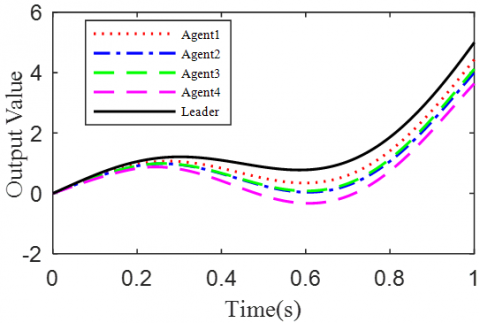
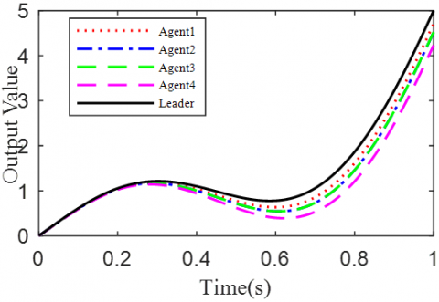
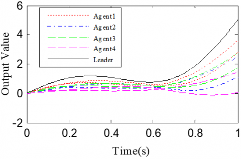
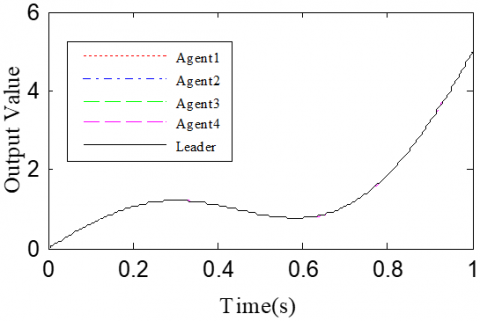
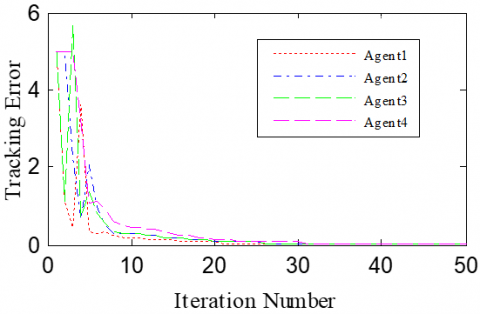
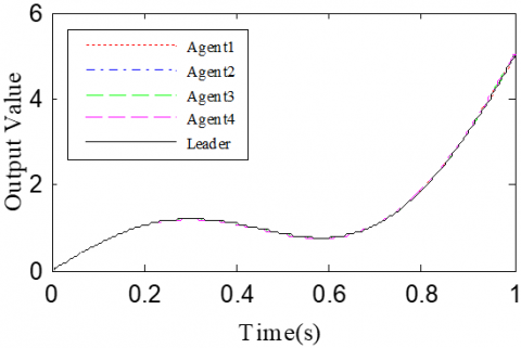
According to the Theorem, the gain matrices were selected as ΓP1=1.2, ΓD1=0.25, ΓP2=1.6, and ΓD2=1.1. Then, we have ρ1=0.876 and ρ2=0.963, which satisfy the conditions in the Theorem. To verify the robustness of open-closed-loop PDα FOILC algorithm to state delay, the delay time was set to 0.1 and 0.5, that is, h=0.1 and h=0.5. The simulation results with h=0.1 and h=0.5 are recorded in Figures 2 and 3, respectively. Figures 2(a)-(c) and 3(a)-(c) present the tracking results in the 5th, 10th, and 50th iterations, respectively; Figure 2(d) and Figure 3(d) show the absolute maximum error of each iteration.
(a) The 5th iteration
(b) The 10th iteration
(c) The 50th iteration
(d) The variation in tracking error
Figure 2. The simulation results with h=0.1s
(a) The 5th iteration
(b) The 10th iteration
(c) The 50th iteration
(d) The variation in tracking error
Figure 3. The simulation results with h= 0.5s
It can be seen that, with the growing number of iterations, each agent gradually tracked the desired trajectory. When h=0.1, the maximum errors of the four followers were 0.0009, 0.0012, 0.0011, and 0.0015 at the 50th iteration, respectively. When h=0.5, the convergence speed was slower than that under h=0.1. Concerning the convergence speed of each agent, agents 1 and 3 converged faster than agents 2 and 4, because the former two can directly receive the information from the leader.
4.2 Case 2: Open-loop PDα FOILC algorithm
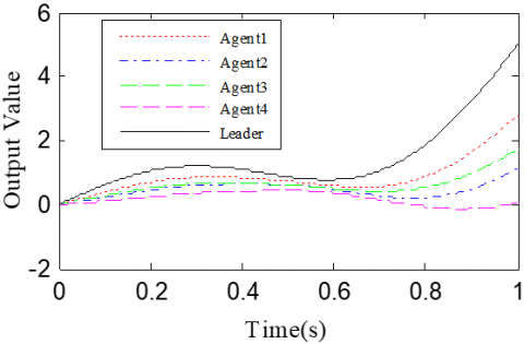
According to Corollary 1 and controller (32), the gain matrices were defined as ΓP1=1.2 and ΓD1=0.25. Similar to Case 1, the delay time was set to 0.1 and 0.5, namely h=0.1 and h=0.5. The simulation results with h=0.1 and h=0.5 are recorded in Figures 4 and 5, respectively. Figures 4(a)-(c) and 4(a)-(c) present the tracking results in the 5th, 10th, and 50th iterations, respectively; Figure 5(d) and Figure 5(d) show the absolute maximum error of each iteration.
It can be seen that, with the growing number of iterations, the multiple agents gradually tracked the desired trajectory. With the increase in delay time, the convergence speed slowed down. In the same iteration, the open-loop PDα FOILC algorithm performed poorer than the open-closed-loop PDα FOILC algorithm. This means the inclusion of the closed-loop control in the latter algorithm improves the control effect and speeds up the convergence.
(a) The 5th iteration
(b) The 10th iteration
(c) The 50th iteration
(d) The variation in tracking error
Figure 4. The simulation results with h= 0.1s
(a) The 5th iteration
(b) The 10th iteration
(c) The 50th iteration
(d) The variation in tracking error
Figure 5. The simulation results with h=0.5s
4.3 Case 3: Closed loop PDα FOILC algorithm
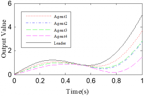
According to Corollary 1 and controller (32), the gain matrices were defined as ΓP2=1.6 and ΓD2=1.1. The initial conditions and delay time were configured the same as Cases 1 and 2. The simulation results with h=0.1 and h=0.5 are recorded in Figures 6 and 7, respectively.
(a) The 5th iteration
(b) The 10th iteration
(c) The 50th iteration
(d) The variation in tracking error
Figure 6. The simulation results with h= 0.1s
(a) The 5th iteration
(b) The 10th iteration
(c) The 50th iteration
(d) The variation in tracking error
Figure 7. The simulation results with h= 0.5s
Figures 6(a)-(c) and 7(a)-(c) present the tracking results in the 5th, 10th, and 50th iterations, respectively; Figure 6(d) and Figure 7(d) show the absolute maximum error of each iteration.
The simulation results show that the closed-loop PDα FOILC algorithm converged slower than the open-closed-loop PDα FOILC algorithm and open-loop PDα FOILC algorithm.
In nature, many physical systems have fractional-order dynamic features. But the integer calculus theory in this research is merely a special case of fractional-order calculus theory. It can only approximate the actual fractional-order system. However, the theory of fractional calculus can reveal the nature of the object truthfully and accurately. The proposed fractional-order controller can achieve a good control performance, which highlights the significance of the research results.
This paper proposes an open-closed-loop PDα FOILC algorithm for FOMAS with state delay. Based on norm theory, graph theory and fractional calculus, the convergence of the proposed algorithm was analyzed in details, and the convergence conditions were summarized. Through theoretical analysis, the proposed algorithm was found to iteratively minimize the error of each agent in FOMAS with state delay. Finally, the algorithm was proved effective through numerical simulation.
[1] Liu, X. (2020). Research on decision-making strategy of soccer robot based on multi-agent reinforcement learning. International Journal of Advanced Robotic Systems, 17(3): 1729881420916960. https://doi.org/10.1177/1729881420916960
[2] Ota, J. (2006). Multi-agent robot systems as distributed autonomous systems. Advanced Engineering Informatics, 20(1): 59-70. https://doi.org/10.1016/j.aei.2005.06.002
[3] Perrusquía, A., Yu, W., Li, X. (2020). Multi-agent reinforcement learning for redundant robot control in task-space. International Journal of Machine Learning and Cybernetics, 1-11. https://doi.org/10.1007/s13042-020-01167-7
[4] Osherenko, A. (2001). Plan Representation and Plan Execution in Multi-agent Systems for Robot Control. In PuK.
[5] Naserian, M., Ramazani, A., Khaki-Sedigh, A., Moarefianpour, A. (2020). Fast terminal sliding mode control for a nonlinear multi-agent robot system with disturbance. Systems Science & Control Engineering, 8(1): 328-338. https://doi.org/10.1080/21642583.2020.1764408
[6] Gu, P., Tian, S. (2019). Consensus tracking control via iterative learning for singular multi-agent systems. IET Control Theory & Applications, 13(11): 1603-1611. https://doi.org/10.1049/iet-cta.2018.5901
[7] Demir, O., Lunze, J. (2014). Optimal and event-based networked control of physically interconnected systems and multi-agent systems. International Journal of Control, 87(1): 169-185. https://doi.org/10.1080/00207179.2013.825816
[8] Liu, X., Zhang, Z., Liu, H. (2017). Consensus control of fractional‐order systems based on delayed state fractional order derivative. Asian Journal of Control, 19(6): 2199-2210. https://doi.org/10.1002/asjc.1493
[9] Liu, J., Chen, W., Qin, K., Li, P. (2018). Consensus of fractional-order multiagent systems with double integral and time delay. Mathematical Problems in Engineering, 2018. https://doi.org/10.1155/2018/6059574
[10] Bensafia, Y., Ladaci, S., Khettab, K., Chemori, A. (2018). Fractional order model reference adaptive control for SCARA robot trajectory tracking. International Journal of Industrial and Systems Engineering, 30(2): 138-156. https://doi.org/10.1504/IJISE.2018.094839
[11] Yu, Z., Jiang, H., Hu, C. (2015). Leader-following consensus of fractional-order multi-agent systems under fixed topology. Neurocomputing, 149: 613-620. https://doi.org/10.1016/j.neucom.2014.08.013
[12] Yu, Z., Jiang, H., Hu, C., Yu, J. (2015). Leader-following consensus of fractional-order multi-agent systems via adaptive pinning control. International Journal of Control, 88(9): 1746-1756. https://doi.org/10.1080/00207179.2015.1015807
[13] Bai, J., Wen, G., Rahmani, A., Chu, X., Yu, Y. (2016). Consensus with a reference state for fractional-order multi-agent systems. International Journal of Systems Science, 47(1): 222-234. https://doi.org/10.1080/00207721.2015.1056273
[14] Ma, X., Sun, F., Li, H., He, B. (2017). The consensus region design and analysis of fractional-order multi-agent systems. International Journal of Systems Science, 48(3): 629-636. https://doi.org/10.1080/00207721.2016.1218570
[15] Yu, W., Li, Y., Wen, G., Yu, X., Cao, J. (2016). Observer design for tracking consensus in second-order multi-agent systems: Fractional order less than two. IEEE Transactions on Automatic Control, 62(2): 894-900. https://doi.org/10.1109/TAC.2016.2560145
[16] Chai, Y., Chen, L., Wu, R., Sun, J. (2012). Adaptive pinning synchronization in fractional-order complex dynamical networks. Physica A: Statistical Mechanics and Its Applications, 391(22): 5746-5758. https://doi.org/10.1016/j.physa.2012.06.050
[17] Sun, M., Wang, D. (2002). Iterative learning control with initial rectifying action. Automatica, 38(7): 1177-1182. https://doi.org/10.1016/S0005-1098(02)00003-1
[18] Sun, M., Ge, S.S., Mareels, I.M. (2006). Adaptive repetitive learning control of robotic manipulators without the requirement for initial repositioning. IEEE Transactions on Robotics, 22(3): 563-568. https://doi.org/10.1109/TRO.2006.870650
[19] Park, K.H. (2005). An average operator-based PD-type iterative learning control for variable initial state error. IEEE Transactions on Automatic Control, 50(6): 865-869. https://doi.org/10.1109/TAC.2005.849249
[20] Meng, D., Jia, Y. (2011). Finite-time consensus for multi-agent systems via terminal feedback iterative learning. IET Control Theory & Applications, 5(18): 2098-2110. https://doi.org/10.1049/iet-cta.2011.0047
[21] Yang, S.P. (2014). On iterative learning in multi-agent systems coordination and control (Doctoral dissertation).