Suman Machavarapu* | Mannam Venu Gopala Rao | Pulipaka Venkata Ramana Rao
© 2020 IIETA. This article is published by IIETA and is licensed under the CC BY 4.0 license (http://creativecommons.org/licenses/by/4.0/).
OPEN ACCESS
The paper presents an adaptive Load Frequency Controller (LFC) based on a neural network for the interconnected multi-area systems. When there is an imbalance between active power generation and demand there will deviation in the frequency from the reference value. Major disturbances that lead to the variation in frequency beyond the allowable limits are variation in load demand and faults, etc. Initially PID based LFC which is a conventional controller is used to bring back the variations in frequency when there is a disturbance. But these conventional controllers will operate certain operating points only, very slow and, are less efficient for nonlinear systems. To avoid the flaws in the conventional controller the artificial intelligent controllers such as neural network and fuzzy logic controllers are designed. The three, two area, and single area systems are considered as the test systems. The response of all the test systems is observed without and with PI, fuzzy, and neural network controllers. It was observed that the neural network controller is outperforming in damping the variation in the frequency due to the disturbances.
backpropagation algorithm, fuzzy logic controller, PI-controller, tie line, load frequency controller, automatic speed governor
Load frequency control (LFC) [1-5] in the electrical industry is a significant issue and the power system has to keep the system frequency and inter-area tie-line power reasonably close as possible to the accepted value for stable, high-quality electrical power. By regulating the plant generator's mechanical input, the frequency can be retained at the reference value. Because of the disturbance such as the load fluctuations and faults, which happens at any time, frequency is disrupted from its rated value. The power system architecture is such that the network frequency and voltage should be kept within tolerable limits. The load frequency controller's main objective is to exercise frequency control as well as real power exchange via outgoing lines. Several methods were proposed for LFC. Although traditional control techniques have been used in most literature, several studies have employed novel and intelligent control techniques as reported in the literature.
Kayalvizhi and Kumar [6] have developed an adaptive fuzzy controller with Model Predictive Control to regulate the frequency of the load. The isolated area with microgrid is considered as the test system the concept of MPC controller and its mathematical equations discussed. The system response was observed without and with PI, MPC, and Fuzzy MPC controllers and, it was identified that the designed controller is providing good results by giving minimum ITSE. Trang and Nouri [7] have modeled a dynamic load frequency controller with the help of limitations of power reserve. Modern power networks will use the three different reserves as the replacement reserves, restoration reserves and, containment reserves. In case of a disturbance inactive power demand and generation, there must be a power reserve to bring back the equilibrium condition. Containment reserve is used in this paper to counteract the variations in frequency due to disturbance.
Farag et al. [8] have proposed a new and control scheme to control load frequency concerning the disturbances. The fractional-order PI controller is used with the Distributed Energy Resource (DER) to counteract the variation in frequency. As a test system two area LFC is chosen. The response of the system was observed with 0.01 p.u step disturbance. It was shown that the proposed method is doing well compared to the fractional-order PI controller.
Manikandan and Kokil [9] have provided a time-varying delay based load frequency controller to damp the variation in frequency due to disturbances. Lyapunov and Krasovskii function analysis is used to identify the system stability. Single area and two area load frequency controllers are considered as the test systems. The Kp and Ki values are determined concerning delay margin to damp the frequency variations.
Pappachen and Fathima [10] have discussed a load frequency controller considering the addition of non-conventional sources into the existing power network. Whatever the sources it may be LFC has to regulate the frequency of load as well as power in the tie line. The working of the LFC technique with a PI controller and with different optimization techniques observed. The fallbacks in the traditional controller and the need for artificial intelligence-based controllers are clearly explained.
In this paper three, two, and single area systems are considered as the test systems. The response of all three test systems is observed without and with different controllers by applying a step input of 0.01 p.u.
The exact reasons why system frequency changes [11] are kept to strict limits are as follows:
Modeling the single area power network comprises of modeling [12] the speed governor, turbine, and generator load model. The speed governor’s governing equations are as given in Eqns. (1) & (2).
$\Delta {{y}_{.E}}(s)=\frac{{{k}_{.1}}*{{k}_{.3}}*{{k}_{c}}*\Delta {{P}_{c.}}(s)-{{k}_{2}}*{{k}_{3.}}*\Delta F(.s)}{{{k}_{4}}+\frac{s}{{{k}_{5}}}}$ (1)
Rearranging the Eq. (1), Eq. (2) will be obtained:
$\Delta .{{Y}_{E}}(.s)=[\Delta {{P}_{C.}}(s)-\frac{1}{R}*\Delta F(s.)]*\frac{{{K}_{sg.}}}{1+{{T}_{sg.}}}$ (2)
where,
$R=\frac{k_{1} * k_{c}}{k_{2}}$= Speed governor speed regulation.
$K_{s g}=\frac{k_{1} * k_{3} * k_{c}}{k_{4}}$= Speed governor gain.
$T_{s g}=\frac{1}{k_{4} * k_{5}}$= Speed governor speed constant.
$\Delta$PC.(s)=Change in steam valve setting.
$\Delta$F(s.)=Change in frequency with respect to disturbance.
$\Delta$Pt(s)=Change in turbine output power.
$\Delta$Pg.(s)=Change in output power of the generator.
$\Delta$Pd.(s)=Change in load demand.
H=Inertia Constant of generator.
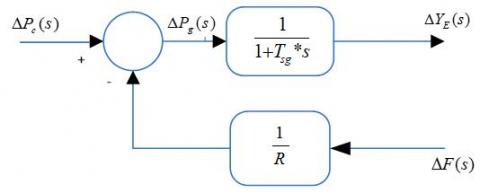
Using Eq. (2) the block diagram of the speed governor will be developed as shown in Figure 1.
Figure 1. Speed governor block diagram
The mathematical equations and the block diagram of the turbine is as given in Eq. (3) and Figure 2.
$\Delta P_{t}(s)=\frac{1}{1+T_{t}^{*} s} * \Delta Y_{e}(s)$ (3)
Figure 2. Turbine block diagram
The equations governing the generator load model are given in Eqns. (4) & (5).
$\Delta F(.s)=\frac{\Delta P_{g .}(s)-\Delta P_{d .}(s)}{B+\frac{2 H}{f^{.0}} * s}$ (4)
Eq. (4) can be rearranged as Eq. (5).
$\Delta F(. s)=\left(\Delta P_{g .}(s)-\Delta P_{. d .}(s)\right) * \frac{K_{p s .}}{1+T_{p s.} *_{s}}$ (5)
where,
$T_{p s}=\frac{2^{*} H}{B^{*} f^{0}}$= Time constant of power system.
$\mathrm{K}_{\mathrm{ps}}=\frac{1}{B}$= Gain of power system.
The Generator Load model block diagram is represented as given in Figure 3.
Figure 3. Generator Load Model block diagram
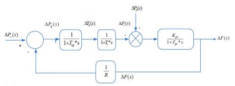
The block diagram of the single area power network can be formed by combining the block diagrams of the speed governor, turbine, and generator load. The full block diagram with a feedback loop is shown in Figure 4.
Figure 4. Single area power network block diagram representation
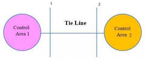
A multi-area system can be formed by interconnecting different control areas. Two different areas interconnected by the tie line is given by given by Figure 5.
Figure 5. Interconnection of two areas with tieline
In multi-area control the goal of the controller is to control the frequency of individual area as well as the tie line power. All the parameters correspond to the first area are represented with suffix 1 and the second area parameters are represented with suffix 2.
The equations governing the two area network is as given in Eqns. (6), (7), (8), (9) and (10).
$\Delta F_{1 .}(s)=\left[\Delta P_{g 1 .}(s)-\Delta P_{d 1 .}(s)-\Delta P_{\text {tie1}}(s)\right] * \frac{K_{p s 1}}{1+T_{p s 1}}$ (6)
$\Delta F_{2}(s)=\left[\Delta P_{g 2 .}(s)-\Delta P_{d 2 .}(s)-\Delta P_{\text {tie2}}(s)\right] * \frac{K_{p s 2}}{1+T_{p s 2}}$ (7)
Let $K_{p s 1}=\frac{1}{B 1}$ and $T_{p s 1}=\frac{2 H_{1}}{B_{1} * f}$
Also,
$\Delta P_{\text {tiel}}=\frac{2 \Pi T_{12.}}{s}\left[\Delta F_{1 .}(s)-\Delta F_{2 .}(s)\right]$ (8)
$\Delta P_{t i e 2}=-\frac{2 \prod a_{12 .} T_{12.}}{s}\left[\Delta F_{1 .}(s)-\Delta F_{2 .}(s)\right]$ (9)
The steady-state error in the tie-line power can be minimized using the PI controller. The area control errors for the two areas can be calculated as given in Eq. (10).
$A C E_{1}(s)=\Delta P_{\text {tie1}}(s)+b_{1} \Delta F_{1}(s)$ (10)
$A C E_{2}(s)=\Delta P_{t i e 2}(s)+b_{2} \Delta F_{2}(s)$ (11)
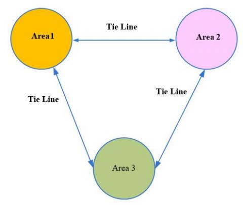
The basic concept of the three Area LFC and its block diagram is as given in Figure 6.
Rarely has the device of a single generator feeding a large and complex area existed in actual life. Many Parallel connected generators may be at a single location, or the load demand of such a wide area would be met at different locations. Wide load areas are split into several small areas, and the interconnected power systems satisfy the load demand accordingly. Power transfer between two areas is done via tie lines.
Figure 6. Three area inter connection
This logic was suggested by Zadeh in the year 1965. Fuzzy logic is a method used in human reasoning to model uncertainty. Fuzzy logic is ideal for intuitively representing ambiguous data and definitions, such as human-language explanation. FLC [13, 14] has potential applications as a control system where human knowledge is intuited using IF and THEN rules by a FIS. Fuzzy's first recorded industrial application was in 1982 that sparked global interest in the industrial and scientific community, as well as the widespread use of fuzzy logic in regression, image processing, prediction, regression, and data analysis. Using fuzzy logic, integrated circuits (ASICs) have been developed for a particular application also.
FL provides a structured method for bringing human knowledge acquired through the experience together. It depends upon three important concepts such as Fuzzy sets, fuzzy set operations, and possibility distributions. Using language expression and using a membership function quantitatively, Fuzzy collection is used to define linguistic variables whose values can be qualitatively represented. Linguistic expressions will help convey ideas and information to humans, while MFs are useful for processing numerical input data.
For control systems, the system inputs are the feedback error i.e. change in frequency and derivation of error i.e. derivation of change in frequency, and the control operation is the output. The architecture of FLC is as given in Figure 7.
Figure 7. Architecture of fuzzy logic controller
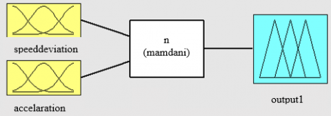
In fuzzification crisp values are converted into the fuzzy membership functions so that FLC can understand. The heart of the system is the Fuzzy Inference System used to imply rules in the rule base on the inputs to produce the output. Two different FIS systems are available such as Sugeno and Mamdani. In this work, the Mamdani FIS system is considered for simulation purposes. The output fuzzy variables again converted to crisp values which are called defuzzification, so that the output also understandable by the common man. Simulation block diagram of FLC is as shown in Figure 8.
Figure 8. Simulation block diagram of the FLC
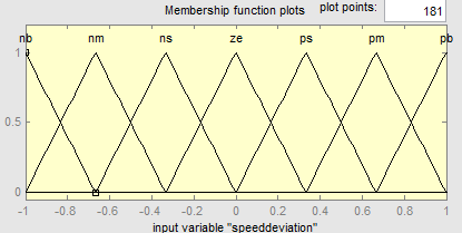
The input membership functions will be the change in frequency and derivation of change in frequency which is as given in Figure 9 and Figure 10.
Figure 9. Membership function of error for a single area fuzzy controller
Figure 10. Membership function of derivative of error for single area fuzzy controller
The rule base which consisting of a set of rules is given in Table 1.
Table 1. Rule base of the fuzzy logic controller
|
DCE |
||||||
|
NB |
NS |
ZZ |
PB |
PS |
||
|
CE |
NB |
S |
S |
M |
M |
B |
|
NS |
S |
M |
M |
B |
VB |
|
|
ZZ |
M |
M |
V |
VB |
VB |
|
|
PB |
M |
B |
VB |
VB |
VVB |
|
|
PS |
B |
VB |
VB |
VVB |
VVB |
|
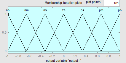
The output membership function of the fuzzy logic controller considered as given in the Figure 11.
Figure 11. Membership function of output for single area fuzzy controller
The ANNs [15, 16] were designed primarily to mimic biological neural networks. ANN's common architectures are single, multi-layer, and feedback neural networks. The backpropagation algorithm is used mainly to train the neural networks of multilayer and feedforward. To obtain the optimized weights it makes use of the slow gradient descent process. The error is the difference between the actual output and the expected output. The generalized delta learning rule or the law of backpropagation is used to adjust the weights in such a way as to eliminate squared error and the actual output is about equal to the expected output. The weights are set according to. The diagram of the backpropagation neural network as given in Figure 12.
Figure 12. Multi-layer feedforward neural network
The Multi-layer network consists of three layers as the input layer contains, I number of neurons, one hidden layer contains J number of neurons, and the output layer contains the number of neurons k. The BPNN algorithm is as provided below:
Step1. Provide inputs (ai) and outputs (bi) patterns.
Step2. Assume that only one hidden layer and initial weight setting are arbitrary, and make a = a(m)=al and b = b(m)=bl.
Step3. Set the input layer unit i activation value to the xi=ai(m).
Step4. The jth Neuron Activation value of hidden layer is calculated as:
$x_{j}^{h}=\sum\limits_{i=1}^{I}{w_{j}^{k}}{{x}_{i}}+w_{oj}^{h}$ (12)
Step5. The jth unit output of the hidden layer is calculated as:
$s_{j}^{h}=f_{j}^{h}(x_{j}^{h})$ (13)
Step6. The kth unit activation value of the output layer,
$x_{k}^{0}=\sum\limits_{i=1}^{I}{w_{kj}^{{}}}x_{j}^{h}+{{w}_{ok}}$ (14)
Step7. The output of the kth neuron in the output layer,
$s_{k}^{0}=f_{k}^{0}(x_{k}^{0})$ (15)
Step8. The kth output unit error term,
$\delta _{k}^{0}=({{b}_{k}}-s_{k}^{0})*\overset{.}{\mathop{f}}\,_{k}^{0}$ (16)
Step9. The weights between hidden and output layers can be calculated as:
${{w}_{kj}}(m+1)={{w}_{kj}}(m)+\eta \delta _{k}^{0}s_{j}^{h}$ (17)
Step10. The Error term at the jth hidden unit is calculated as
$\delta _{j}^{h}=\overset{.}{\mathop{f}}\,_{j}^{h}\sum\limits_{k=1}^{K}{\delta _{k}^{0}}{{w}_{kj}}$ (18)
Step11. The weights between input and hidden layer can be updated as:
$w_{ji}^{h}(m+1)=w_{ji}^{h}(m)+\eta \delta _{j}^{h}{{a}_{i}}$ (19)
Step12. The error for the lth pattern can be calculated as ${{E}_{l.}}=\frac{1}{2}\sum\limits_{k=1}^{K.}{({{b}_{lk.}}}-s_{k}^{0.}{{)}^{2}}$ and total error calculates as:
$E=\sum\limits_{l=1.}^{L.}{{{E}_{l}}}$ (20)
Step13. All the patterns are applied one by one and the weights are changed till the error is minimized.
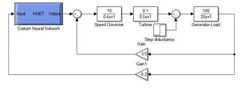
The frequency deviation of the single area system was observed without and with PI, fuzzy, and Backpropagation neural network controllers. The single area Load frequency control with the Backpropagation neural network is as given in Figure 13.
The response of the single area system without and with different controllers is as given in Figure 13 to Figure 17.
The comparison table of peak values and settling times of the single area system is as given in Table 2.
Table 2. Comparison of performance of controllers on single area
|
S. No |
Controller |
Peak Overshoot |
Settling time |
|
1 |
Without |
-0.0475 |
Never settles at zero |
|
2 |
PI |
-0.045 |
27 |
|
3 |
Fuzzy |
-0.027 |
17.5 |
|
4 |
BPNN |
-0.0265 |
15.8 |
Figure 13. Single area neural network LFC
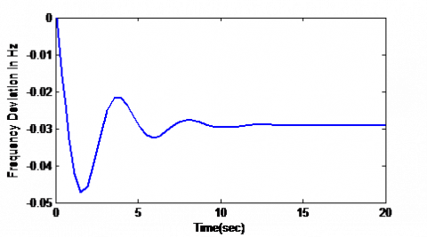
Figure 14. Single area LFC without the controller
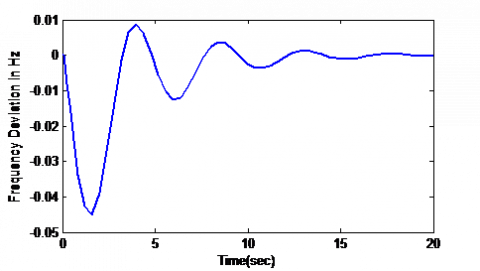
Figure 15. Single area LFC with PI controller
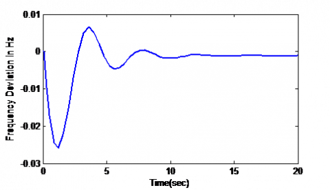
Figure 16. Single area LFC with FLC
Figure 17. Single are LFC with the Back propagation neural network controller
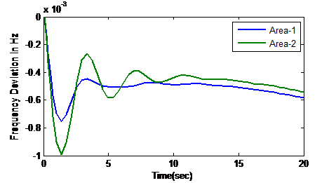
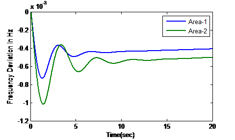
Figure 18. Two area LFC without the controller
Figure 19. Two area LFC with PI controller
Figure 20. Two area LFC with FLC
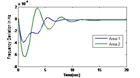
Figure 21. Two area LFC with the back propagation neural network controller
Figure 22. Three area LFC without the controller
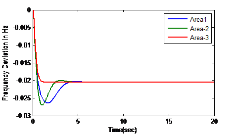
Figure 23. Three area LFC with PI controller
Figure 24. Three area LFC with the fuzzy controller
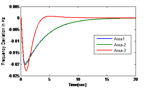
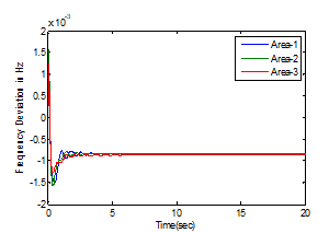
Figure 25. Three area LFC with the Back propagation neural network controller
Table 3. Comparison of performance of controllers on two area
|
Area |
Controller |
Peak Overshoot |
Settling time |
|
1 |
Without |
-0.055 |
Never settles at zero |
|
PI |
-0.0007 |
26 |
|
|
Fuzzy |
0.00065 |
18 |
|
|
BPNN |
-0.0004 |
16.5 |
|
|
ELMNN |
0.00038 |
15.4 |
|
|
2 |
Without |
-0.051 |
Never settles at zero |
|
PI |
-0.001 |
26.5 |
|
|
Fuzzy |
0.00095 |
17.8 |
|
|
BPNN |
0.00063 |
16 |
|
|
ELMNN |
0.00061 |
15 |
Table 4. Comparison of performance of controllers on two area
|
Area |
Controller |
Peak Overshoot |
Settling time |
|
1 |
Without |
-0.027 |
Never settled to zero |
|
PI |
-0.019 |
31 |
|
|
Fuzzy |
-0.017 |
10.5 |
|
|
BPNN |
-0.015 |
9.8 |
|
|
ELMNN |
-0.011 |
9.5 |
|
|
2 |
Without |
-0.0275 |
Never settled to zero |
|
PI |
-0.02 |
30.5 |
|
|
Fuzzy |
-0.0174 |
10.2 |
|
|
BPNN |
-0.0155 |
9.2 |
|
|
ELMNN |
-0.0125 |
9.1 |
|
|
3 |
Without |
-0.026 |
Never settled to zero |
|
PI |
-0.024 |
30.1 |
|
|
Fuzzy |
-0.0184 |
8.5 |
|
|
BPNN |
-0.0165 |
8.2 |
|
|
ELMNN |
-0.013 |
8 |
The performance of different controllers observed with two area test system also. The Figures 18 to 21 shows the response of different controllers.
The three area test system response also observed with the different controllers which are given in Figure 22 to 25.
The performance comparison of different controllers of two are system is given in Table 3.
The performance comparison of different controllers of two are system is given in Table 4.
The deviation in frequency was observed with 0.01 p.u step disturbance without and with PI, Fuzzy and Neural network controller for a single area, two area, and three area power systems. The peak value and the settling time were observed with all controllers for different test systems. For example, consider the single area system without the LFC controller the peak value will be -0.045 Hz and it doesn’t settle back to zero. The PI controller can bring back the peak value to -0.045 Hz and the settling time to 27 sec. The fuzzy controller can control the Peak value to -0.027 Hz and the settling time 17.5 sec. The peak value and the settling time will be -0.0265Hz and the 15.6 sec with Backpropagation neural network controller. In the single area system, controller to controller the response is improving and there will be best results with the Backpropagation neural network controller. Like this in the remaining two area and three area systems the proposed system is outperforming compared to the remaining controller.
[1] Ranganayakulu, R., Babu, G.U., Rao, A.S., Patle, D.S. (2016). A comparative study of fractional order PI/PID tuning rules for stable first order plus time delay processes. Resource-Efficient Technologies, 2: S136-S152. https://doi.org/10.1016/j.reffit.2016.11.009
[2] Annamraju, A., Nandiraju, S. (2019). Robust frequency control in a renewable penetrated power system: An adaptive fractional order-fuzzy approach. Protection and Control of Modern Power Systems, 4(16). https://doi.org/10.1186/s41601-019-0130-8
[3] Liu, H., Hu, Z., Song, Y. (2015). Vehicle-to-grid control for supplementary frequency regulation considering charging demands. IEEE Transactions on Power Systems, 30(6): 3110-3119. https://doi.org/10.1109/TPWRS.2014.2382979
[4] Debbarma, S., Dutta, A. (2017). Utilizing electric vehicles for LFC in restructured power systems using fractional order controller. IEEE Transactions on Smart Grid, 8(6): 2554-2564. https://doi.org/10.1109/TSG.2016.2527821
[5] Hanwate, S., Hote, Y.V., Saxena, S. (2018). Adaptive policy for load frequency control. IEEE Transactions on Power Systems, 33(1): 1142-1144. https://doi.org/10.1109/TPWRS.2017.2755468
[6] Kayalvizhi, S., Kumar, D.M.V. (2017). Load frequency control of an isolated micro grid using fuzzy adaptive model predictive control. IEEE Access, 5: 16241-16251. https://doi.org/10.1109/ACCESS.2017.2735545
[7] Trang, L.T.M., Nouri, H. (2018). Modeling dynamic frequency control with power reserve limitations. 53rd International Universities Power Engineering Conference, Glasgow, UK, pp. 1-5. https://doi.org/10.1109/UPEC.2018.8541972
[8] Farag, K.A., Sharaf, A.M. (2019). A novel modified robust load frequency controller scheme. Energy Systems. https://doi.org/10.1007/s12667-019-00341-3
[9] Manikandan, S., Kokil, P. (2019). Delay-dependent stability analysis of network-based load frequency control of one and two area power system with time-varying delays. Fluctuation and Noise Letters, 18(1): 1-19. https://doi.org/10.1142/S021947751950007X
[10] Pappachen, A., Fathima, A.P. (2017). Critical research areas on load frequency control issues in a deregulated power system: A state-of-the-art-of-review. Renewable and Sustainable Energy Reviews, 72: 163-177. https://doi.org/10.1016/j.rser.2017.01.053
[11] Suman, M., Rao, M.V.G., Kumar, G.R.S.N., Sekhar, O.C. (2014). Load frequency control of three unit interconnected multimachine power system with PI and fuzzy controllers. 2014 International Conference on Advances in Electrical Engineering (ICAEE), Vellore, India, pp. 1-5. https://doi.org/10.1109/ICAEE.2014.6838530
[12] Bharti, K., Singh, V.P., Singh, S.P. (2020). Impact of intelligent demand response for load frequency control in smart grid perspective. IETE Journal of Research, 1-12. https://doi.org/10.1080/03772063.2019.1709570
[13] Prakash, S., Sinha, S.K. (2011). Application of artificial intelligence in load frequency control of interconnected power system. International Journal of Engineering, Science and Technology, 39(4): 264-275. https://doi.org/10.4314/ijest.v3i4.68558
[14] Lal, D.K., Barisal, A.K. (2019). Combined load frequency and terminal voltage control of power systems using moth flame optimization algorithm. Journal of Electrical Systems and Information Technology, 6(8): 1-24. https://doi.org/10.1186/s43067-019-0010-3
[15] Khamari, D., Rout, J.K. (2019). Load frequency control of two area power system using PID1 controller. International Journal of Engineering Research & Technology (IJERT), 8(3): 245-248. https://doi.org/10.1177/2F1077546316634562
[16] Tungadio, D.H., Sun, Y.X. (2019). Load frequency controllers considering renewable energy integration in power system. Energy Reports, 5: 436-454. https://doi.org/10.1016/j.egyr.2019.04.003