Wentang Wang* | Kun Tian | Jianxia Zhang
© 2020 IIETA. This article is published by IIETA and is licensed under the CC BY 4.0 license (http://creativecommons.org/licenses/by/4.0/).
OPEN ACCESS
The active suspension system of automobiles has great advantages in riding comfort and handling stability. However, it is a challenging task to design an active control method for this system, owing to system features like multi-input and multi-output, time variation, and nonlinearity. To cope with the challenge, this paper mathematically models the active suspension system based on the full-car model, rather than the common quarter car model, and obtains a nonlinear dynamic model with variables like displacement, roll angle and pitch angle. Subsequently, an incremental proportional–integral–derivative (PID) controller was designed, and a deep reinforcement learning adaptive (DRLA) controller was proposed to realize online adjustment of control parameters. Finally, the active suspension system of the entire vehicle was simulated on MATLAB/Simulink. The simulation results prove that the DRLA controller can effectively reduce the displacement, the amplitude of roll and pitch angle of the car body, and greatly enhance the smoothness of the ride on the vehicle.
active suspension system, reinforcement learning (RL), adaptive control, dynamic modelling
Recent years has witnessed great improvement to the riding, handling and safety of road vehicles, thanks to the extensive explorations into the design of automotive suspension system [1-3]. In the suspension system, multiple springs and dampers connect the vehicle body with the wheels, and thereby control the vertical motions of the vehicle body. The main functions of the system include offsetting the variation in the force and payload of the vehicle body induced by turning, acceleration or braking, and isolates the passenger cabin from the irregularities on road.
Automotive suspension systems can be divided into passive suspension system, semi-active suspension system, and active suspension system. The passive suspension system solely relies on its own structure to damp the vibrations resulted from road disturbances, without needing any external control force. The damping coefficient of the system is almost constant. The classic semi-active suspension system has a variable damping coefficient, and realizes electronic modulation by magnetorheological (MR), electrorheological (ER) or electro-hydraulic techniques. The active suspension system applies the control force based on the real-time state feedback of the vehicle, achieving a good vibration damping effect, and assists with the attitude control of the car body.
Many scholars have attempted to design an effective automotive suspension system. For example, Spelta et al. [4] proposed a new comfort-oriented variable damping and stiffness control algorithm, named stroke–speed–threshold–stiffness–control, which overcomes the critical tradeoff between the choice of the stiffness coefficient and the end-stop hitting; the variable-damping and-stiffness suspension, coupled with this algorithm, achieves much better comfort performance than traditional passive suspensions and more classical variable-damping semi-active suspensions. Bei et al. [5] built a full-car model based on multi-body dynamics, including the steering system, front and rear suspensions, tire, driving controller, and road, and verified the model through tests. Based on co-simulation, a controller was created based on hybrid sensor network control. The principle of the controller switches among comfort controller, stability controller, and safety controller, according to working conditions. The controller effectively improves the ride comfort, handling stability, and driving safety.
Recently, there is a substantial growth in the research and development of the active suspension systems of car models. To improve ride comfort and road handling, the active suspension controls vehicle attitude and reduces the impact of road roughness by increasing and dissipating system energy through the actuator. The active suspension system is a closed-loop system, in which the required actuator force can be predicted based on the suspension travel [6]. Considering the vibrations acting on human body in the vertical direction, Rao and Anusha, [7] carried out bump analysis on a three degrees-of-freedom (3DOF) quarter car model, controlled the active suspension of the model with fuzzy logic, and simulated the transient response to road perturbations. Sun et al. [8] constructed a full-car model with high nonlinearity, selected actuator forces as virtual inputs to suppress disturbance, and designed controllers that help real force inputs track virtual ones, based on the adaptive H∞ robust control technique.
In addition, Yao et al. [9] presented a method for controlling an automobile to tilt toward the turning direction using active suspension: the desired tilt angle was determined through dynamic analysis, and used to establish an active tilt sliding mode controller, which causes zero steady-state tilt angle error; finally, the effectiveness of the controller was confirmed through simulation. Na et al. [10] put forward an active suspension control of full-car systems with unknown nonlinearity; on the upside, this control method can handle the uncertainties and nonlinearities in the systems, without using any function approximator or online adaptive function; on the downside, the method poses high requirements on the accuracy of model parameters. Gang [11] developed a full-car model with unknown dynamics and uncertain parameters, and designed a novel non-singular terminal sliding mode controller (NSTSMC), which can stabilize the vertical, pitch, and roll displacements into a desired equilibrium in finite time. However, the parameters of the controller must be adjusted, if any change takes place to the model.
In most of the above methods, the control parameters must be adjusted to suit the parameter changes of the car model. This obviously limits the application scope of the control algorithm. The reinforcement learning (RL) is an emerging method that adaptively adjusts control parameters, according to environmental feedbacks and given rewards. The RL is an important tool of machine learning (ML), whose initial focuses include pattern classification, supervised learning and adaptive control. After assigning the learning agent a goal, the RL proceeds through repeated interactions with the dynamic environment, that is, mapping situations (states) to actions [12-14]. The mapping from the action in a state to the scalar number of the reward constitutes the immediate demand of the state. The RL is an algorithm that can effectively find the optimal value function. The learning agent learns its environment through exploration, and gains experience in this process [15-19]. Suffice it to say that the RL provides a suitable tool for active control of automotive suspension system.
Targeting automobile active suspension system, this paper first models the nonlinear dynamics of the entire vehicle, setting up the control target for the design of the controller. Then, an incremental proportional–integral–derivative (PID) controller was developed to realize the target. Since the control parameters cannot automatically adapt to environmental changes, the authors proposed a deep RL adaptive (DRLA) controller based on adaptive critic element (ACE) and associative search element (ASE), and applied the DRLA controller to update control parameters online in real time. Finally, the DRLA controller was fully verified through simulations on MATLAB/Simulink.
The remainder of this paper is organized as follows: Section 2 puts forward the dynamic model of the whole vehicle; Section 3 designs the DRLA controller based on the RL algorithm; Section 4 compares the effect of the DRLA controller with that of the PID controller; Section 5 gives the conclusions and looks forward to the future research.
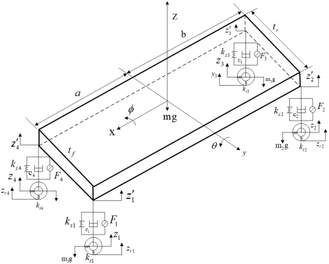
The 7DOF full-car model, including the car body and four wheels, is illustrated in Figure 1, where m is the mass of the car body; m1, m2, m3, and m4 are the masses of the four wheels, respectively; z1, z2, z3, and z4 are the vertical displacements of the four wheels, respectively; $z_{1}^{\prime}, z_{2}^{\prime}, z_{3}^{\prime}$ and $z_{4}^{\prime}$ are the vertical displacements at the four corners of the car body, respectively; ksi, ci, and Fi(i=1,⋯,4) are the stiffness, damping coefficient, and actuator force (active control force) of the springs at the four corners of the car body; θ and ϕ are the pitching and rolling of the car body, respectively; zr1, zr2, zr3, and zr4 are the road displacements of the four wheels, respectively; z is the heave of the car body; a and b are the distances to the front and the rear from the centroid, respectively; tf and tr are the front and rear treads, respectively. The 7DOFs of the full-car model include zr1, zr2, zr3, zr4, z, θ, and ϕ.
Figure 1. Full-car model of the active suspension system
The actuators are arranged vertically between the mass of the car body and that of the wheels, providing the control force to the active suspension system. The full-car model makes it possible to measure the pitching and rolling of the car body, which cannot be measured in the quarter car model of the vehicle suspension system. Here, a hydraulic actuator is placed on each suspension between the spring and non-spring. The dynamic features of the actuator were neglected in the simulation of the full-car model.
Using the schematic diagram of the full-car model, the motion equations of the model [20, 21] were derived from Newton’s second law of motion. The heave, pitch angle, and roll angle can be respectively defined as:
$I_{r} \ddot{\varphi}=-b_{1} t_{f}\left(\dot{z}_{1}-\dot{z}_{u 1}\right)+b_{2} t_{f}\left(\dot{z}_{2}-\dot{z}_{u 2}\right)-b_{3} t_{r}\left(\dot{z}_{3}\right.$
$\left.-\dot{z}_{u 3}\right)+b_{4} t_{r}\left(\dot{z}_{4}-\dot{z}_{u 4}\right)$
$-k_{1} t_{f}\left(z_{1}-z_{u 1}\right)+k_{2} t_{f}\left(z_{2}\right.$
$\left.-z_{u 2}\right)-k_{3} t_{r}\left(z_{3}-z_{u 3}\right)$
$+k_{4} t_{r}\left(z_{4}-z_{u 4}\right)+t_{f} u_{1}-t_{f} u_{2}$
$+t_{r} u_{3}-t_{r} u_{4}$ (1)
$\begin{aligned} I_{p} \ddot{\theta}=-b_{1} a\left(\dot{z}_{1}-\dot{z}_{u 1}\right)-b_{2} a\left(\dot{z}_{2}-\dot{z}_{u 2}\right) \\ &+b_{3} a\left(\dot{z}_{3}-\dot{z}_{u 3}\right)+b_{4} b\left(\dot{z}_{4}-\dot{z}_{u 4}\right) \\ &-k_{1} a\left(z_{1}-z_{u 1}\right)-k_{2} a\left(z_{2}-z_{u 2}\right) \\ &+k_{3} b\left(z_{3}-z_{u 3}\right)+k_{4} b\left(z_{4}-z_{u 4}\right) \\ &+a u_{1}+a u_{2}+a u_{3}+a u_{4} \end{aligned}$ (2)
$\begin{aligned} m_{s} \ddot{z}=-b_{1}\left(\dot{z}_{1}-\dot{z}_{u 1}\right)-b_{2}\left(\dot{z}_{2}-\dot{z}_{u 2}\right)-b_{3}\left(\dot{z}_{3}\right.\\\left.-\dot{z}_{u 3}\right)-b_{4}\left(\dot{z}_{4}-\dot{z}_{u 4}\right)-k_{1}\left(z_{1}\right.\\\left.-z_{u 1}\right)-k_{2}\left(z_{2}-z_{u 2}\right)-k_{3}\left(z_{3}\right.\\-z_{u 3} &-k_{4}\left(z_{4}-z_{u 4}\right)+u_{1}+u_{2} \\+u_{3}+u_{4} \end{aligned}$ (3)
Under external disturbances, the vertical motions of tires at the four corners can be respectively described:
$m_{u_{1}} \ddot{z}_{u 1}=b_{1}\left(\dot{z}_{1}-\dot{z}_{u 1}\right)+k_{1}\left(\dot{z}_{1}-\dot{z}_{u 1}\right)+k_{t 1}\left(z_{r i}-z_{u 1}\right)-u_{1}$ (4)
$m_{u 2} \ddot{z}_{u 2}=b_{2}\left(\dot{z}_{2}-\dot{z}_{u 2}\right)+k_{2}\left(z_{2}-z_{u 2}\right)+k_{t 2}\left(z_{r 2}-z_{u 2}\right)-u_{2}$ (5)
$m_{u 3} \ddot{z}_{u 3}=b_{3}\left(\dot{z}_{3}-\dot{z}_{u 3}\right)+k_{3}\left(z_{3}-z_{u 3}\right)+k_{t 3}\left(z_{r 3}-z_{u 3}\right)-u_{3}$ (6)
$m_{u_{4}} \ddot{z}_{u 4}=b_{4}\left(\dot{z}_{4}-\dot{z}_{u 4}\right)+k_{4}\left(z_{4}-z_{u 4}\right)-k_{t 4}\left(z_{r 4}-z_{u 4}\right)-u_{4}$ (7)
The vertical displacements of corners 1-4 can be respectively expressed by the heave, pitch angle, and roll angle:
$z_{1}=z+t_{f} \phi_{s}+a \theta_{s}, \dot{z}_{1}=\dot{z}+t_{f} \dot{\phi}_{s}+a \dot{\theta}_{s}$ (8)
$z_{2}=z+t_{f} \phi_{s}+a \theta_{s}, \dot{z}_{2}=\dot{z}-t_{f} \dot{\phi}_{s}+a \dot{\theta}_{s}$ (9)
$z_{3}=z+t_{f} \phi_{s}+a \theta_{s}, \dot{z}_{3}=\dot{z}+t_{r} \dot{\phi}_{s}-b \dot{\theta}_{s}$ (10)
$z_{4}=z+t_{f} \phi_{s}+a \theta_{s}, \dot{z}_{4}=\dot{z}-t_{r} \dot{\phi}_{s}-b \dot{\theta}_{s}$ (11)
This section designs an incremental PID controller, and the DRLA controller for active control the suspension system. The incremental PID controller was designed as a control sample to demonstrate the superiority of the DRLA controller.
3.1 Incremental PID controller
The traditional PID controller contains a proportional link P(e(t)), an integral link I(e(t)), and a differential link D(e(t)) [20]. Suppose each wheel is completely decoupled and independently controlled by the active control force Fi(t). Then, the control input Fi(t) can be expressed as:
$F_{i}(t)=K_{P} e(t)+K_{I} \int e(t) d t+K_{D} \frac{d e(t)}{d t}$ (12)
where, KP, KI, and KD are proportional, integral, and differential factors, respectively; e(t) is the control error:
$e(t)=z_{i}(t)-z_{d}(t)$ (13)
where, zd(t) is the control target; zi(t) is the actual response. The PID parameters were tuned by the Zeigler–Nicholds method.
Then, the traditional PID was extended into an incremental PID capable of deep RL and adaptive adjustment:
$F_{i}(t)=F_{i}(t-1)+\Delta F_{i}(t)=F_{i}(t-1)+K_{P} e(t)+K_{I} \Delta e(t)+K_{D} \Delta^{2} e(t)$ (14)
where, Δe(t)=e(t)-e(t-1), and Δ2e(t)=e(t)-2*e(t-1)+e(t-2).
Figure 2. The structure of incremental PID controller
The structure of the incremental PID controller is explained in Figure 2. Compared with the traditional PID controller, the incremental PID controller saves storage space for deep RL, remains robust to environmental rewards, and improves the RL rate.
3.2 DRLA controller
The DRLA controller was designed by adaptively updating the parameters of the incremental PID controller online through deep RL. The structure of the DRLA controller is presented in Figure 3.
The RL control system has two main functional components, namely, the ASE, and the ACE. The ASE attempts to find the best action in a given system state through trial and error or through generation and test search, that is, mapping the state vector into the KP, KI, and KD of the PID controller. The ACE receives reinforcement signals from its environment, and then generates internal RL signals for ASE adjustment.
The Actor network has n paths for non-enhanced signal input, a path for enhanced input, and a path for signal output. Let {xi (t),1≤i≤n} be the real-valued signal on the i-th path for unenhanced input, and y(t) be the output at time t. Then, the ASE output can be defined as:
$y(t)=f\left(\sum_{i} w_{i}(t) x_{i}(t)+\text { noise }(t)\right)$ (15)
where, noise(t) is a real-valued random variable obeying zero mean Gaussian distribution, with covariance as the probability function; f(x, t) is an S-type function or a threshold function; wi is a weight that is updated based on internal enhancement r'(t) and the legal input ei(t) in the i-th path:
$w_{i}(t+1)=w_{i}(t)+\alpha r^{\prime}(t) e_{i}(t)$ (16)
where, α is the learning rate; ei(t) is the legal exponential decay curve with time:
$e_{i+1}(t)=\delta e_{i}(t)+(1-\delta) y(t) x_{i}(t)$ (17)
where, (0≤δ≤1) is the decay rate.
The final enhancement as predicted can be described as a linear function of the input vector x in the Critic network:
$p(t)=\sum_{i} v_{i}(t) x_{i}(t)$ (18)
The p(t) will converge to the accurate prediction by updating the weight vi as follows:
$v_{i}(t+1)=v_{i}(t)+\beta[r(t)+\gamma p(t)-p(t-1)] \bar{x}$ (19)
where, β is the learning rate; r(t) is the enhanced signal provided by the system environment; $\bar{x}(t)$ is the trajectory of the input vector xi(t); 0≤γ≤1 is a positive value. Without external enhancement, the prediction of the positive state quantity will weaken. In other words, heuristic or internal enhancement r' encompasses the change of p value and the external reinforcement. The farther the future value of p is from the current state of the system, the higher its discount rate, and the trajectory $\bar{x}$ behaves more similar to the legal trajectory ei defined in formula (17). However, as long as there is a nonzero signal on a path, the input path will be qualified no matter what is the role of the element. $\bar{x}$ can be calculated by the following linear difference equation:
$\bar{x}_{i}(t+1)=\eta \bar{x}_{i}(t)+(1-\eta) \bar{x}_{i}(t)$ (20)
where, 0≤η≤1 is the trajectory decay rate. According to formula (20), as long as the sum of actual reinforcement r(t) and the current prediction p(t) differs from the prediction p(t-1) for this sum, the weight of the qualified path will change. Then, a learning rule was provided to find the weight such that p(t-1) approximates r(t)+γp(t). The ACE output is an improved or internally enhanced signal:
$r^{\prime}(t)=r(t)+\gamma p(t)-p(t-1)$ (21)
This is also known as a time difference (TD) error. The parameters should be adjusted to reduce the TD between successive states. The reward function can be defined as:
$R(t)=\zeta r(t)$ (22)
Figure 3. The structure of the DRLA controller
Two simulations were carried out on MATLAB/Simulink, which applies to linear and non-linear systems that contain both continues and discrete data, as well as systems with multiple sampling frequencies. The model parameters of the automobile active suspension system are configured as shown in Table 1.
Table 1. The model parameters of the automobile active suspension system
|
m |
1,020kg |
|
m1=m2=m3=m4 |
15 kg |
|
ks1=ks4 |
22,000 N/m |
|
ks2=ks3 |
19,000N/m |
|
c1=c2=c3=c4 |
800Ns/m |
|
kt1=kt2=kt3=kt4 |
143,000 N/m |
|
a |
1.025m |
|
b |
2.204 m |
|
tr |
0.612 m |
|
tf |
0.85 m |
|
Ir |
1,859 kg m2 |
|
Ip |
471kg m2 |
|
g |
9.81 kg m2 |
4.1 Simulation 1
Simulation 1 was carried out on a continuously changing road surface. To make the simulation more realistic, the amplitude and frequency of surface changes were set to 0.02cm and 2.5Hz, respectively; the road surface was obtained by zr(t) = 0.02 sin(5πt).
To avoid redundancy, only the simulation data on wheel 1 and corner 1 were analyzed (Figures 4-6). Figures 7-9 compares the online adaptive adjustments of the PID parameters by the incremental PID controller and the DRLA controller.
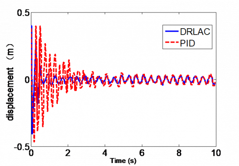
Figure 4. Vertical displacement of wheel 1 (m)
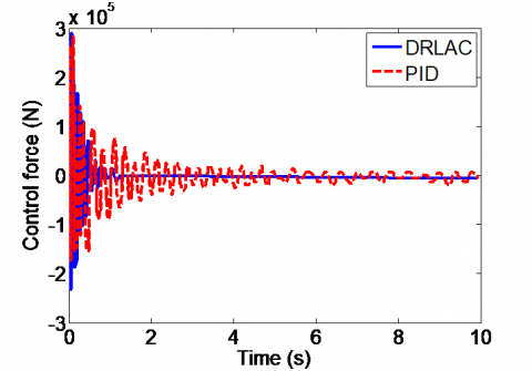
Figure 5. Active control force of wheel 1
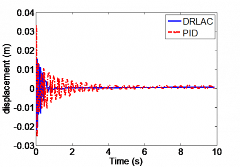
Figure 6. Vertical displacement of corner 1
Figure 7. Adaptive change of KP
Figure 8. Adaptive change of KI
Figure 9. Adaptive change of KD
As shown in Figure 4, under the incremental PID controller, the vertical displacement of wheel 1 did not stabilize until 5.8s; the vibration amplitude peaked at 0.45m. Under the DRLA controller, the vertical displacement of wheel 1 stabilized at 1.2s; the vibration amplitude, which was high at the initial moment, decreased to and stabilized at 0.1m. Hence, the DRLA controller led to faster response.
As shown in Figure 5, under the incremental PID controller, the control force fluctuated significantly and kept oscillating. Under the DRLA controller, the control force changed slowly and stabilized at 1.5s.
As shown in Figure 6, under the incremental PID controller, the vertical displacement of corner 1 kept oscillating, exhibiting significant changes. Under the DRLA controller, the vertical displacement of corner 1 changed less significantly, and quickly stabilized at 1.3s.
4.2 Simulation 2
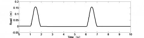
The responses of pitch angle and roll angle were simulated on the road in Figure 10. The simulation results are displayed in Figures 11-12. The RL rewards are given in Figure 13.
Figure 10. Time-domain spectrum of the road
Figure 11. Dynamic responses of pitch angle
Figure 12. Dynamic responses of roll angle
Figure 13. The curves of RL rewards
As shown in Figure 11, the pitch angle of corner 1 changed more significantly and responded slower under the incremental PID controller than under the DRLA controller.
As shown in Figure 12, the roll angle of corner 1 changed by 2.8deg at the maximum under the incremental PID controller, and 1.8deg at the maximum under the DRLA controller; the stabilization time of the roll angle under the incremental PID controller was 2s longer than that under the DRLA controller.
The simulation data on the other three wheels are listed in Table 2. Judging by the root mean square (RMS) values, the DRLA controller outperformed the incremental PID controller.
Table 2. Root mean squared value of suspension system
|
Position |
Parameter |
RMS value |
|
|
Incremental PID controller |
DRLA controller |
||
|
Corner 2 |
Displacement (m) |
6.75 |
3.83 |
|
Pitch angle (deg) |
1.35 |
0.95 |
|
|
Roll angle (deg) |
1.10 |
0.92 |
|
|
Corner 3 |
Displacement (m) |
6.45 |
3.62 |
|
Pitch angle (deg) |
1.27 |
0.94 |
|
|
Roll angle (deg) |
1.05 |
0.91 |
|
|
Corner 4 |
Displacement (m) |
6.53 |
3.65 |
|
Pitch angle (deg) |
1.30 |
0.98 |
|
|
Roll angle (deg) |
1.08 |
0.94 |
|
The suspension based on the 7-DOF full-car model has strong nonlinearly. The actuators of active control add to the complexity of the mathematical model on the active suspension system. In the active suspension system, the model-based controller has poor real-time performance, due to the nonlinear features of its actuators. Based on the deep RL strategy of ACE and ASE, this paper designs the DRLA controller by adaptively adjusting the incremental PID controller. The simulation results show that:
Under the incremental PID controller, the displacement response kept oscillating, and the vertical displacement changed significantly. Under the DRLA controller, the displacement response changed less significantly, and stabilized quickly at 1.3s.
Under the incremental PID controller, the pitch angle of corner 1 changed significantly by 3.7deg, and took 4s to stabilize. Under the DRLA controller, that pitch angle changed by 2.8deg only, and took merely 3.2 to stabilize.
Under the incremental PID controller, the roll angle changed by 2.8deg at the maximum. Under the DRLA controller, the roll angle changed by 1.8deg at the maximum. Besides, the roll angle stabilized 2s faster under the DRLA controller than the incremental PID controller.
The RMS values of all wheels indicate that the DRLA controller outshined the incremental PID controller in both vibration amplitude and the time to reach stability.
To sum up, the DRLA controller can greatly improve the riding comfort of passengers and the operability of the vehicle. The future research will further verify the proposed DRLA controller through experiments on full-scale experimental platform.
This research was supported by the Key scientific and technological project of Henan Province (Grant No.: 172102210123); The Key scientific research project plan of colleges and universities in Henan Province (Grant No.: 20B590001).
[1] Eski, I., Yıldırım, Ş. (2009). Vibration control of vehicle active suspension system using a new robust neural network control system. Simulation Modelling Practice and Theory, 17(5): 778-793. https://doi.org/10.1016/j.simpat.2009.01.004
[2] Wang, G., Chadli, M., Chen, H., Zhou, Z. (2019). Event-triggered control for active vehicle suspension systems with network-induced delays. Journal of the Franklin Institute, 356(1): 147-172. https://doi.org/10.1016/j.jfranklin.2018.10.012
[3] Youn, I., Khan, M.A., Uddin, N., Youn, E., Tomizuka, M. (2017). Road disturbance estimation for the optimal preview control of an active suspension systems based on tracked vehicle model. International Journal of Automotive Technology, 18(2): 307-316. https://doi.org/10.1007/s12239-017-0031-7
[4] Spelta, C., Previdi, F., Savaresi, S.M., Bolzern, P., Cutini, M., Bisaglia, C., Bertinotti, S.A. (2011). Performance analysis of semi-active suspensions with control of variable damping and stiffness. Vehicle System Dynamics, 49(1-2): 237-256. https://doi.org/10.1080/00423110903410526
[5] Bei, S., Huang, C., Li, B., Zhang, Z. (2020). Hybrid sensor network control of vehicle ride comfort, handling, and safety with semi-active charging suspension. International Journal of Distributed Sensor Networks, 16(2): 1-10. https://doi.org/10.1177/1550147720904586
[6] Sivakumar, K., Kanagarajan, R., Kuberan, S. (2018). Fuzzy control of active suspension system using full car model. Mechanics, 24(2): 240-247. https://doi.org/10.5755/j01.mech.24.2.17457
[7] Rao, T.R., Anusha, P. (2013). Active suspension system of a 3 DOF quarter car using fuzzy logic control for ride comfort. International Conference on Control and Automation, pp. 1-6. https://doi.org/10.1109/CARE.2013.6733771
[8] Sun, W., Gao, H., Yao, B. (2013). Adaptive robust vibration control of full-car active suspensions with electrohydraulic actuators. IEEE Transactions on Control Systems Technology, 21(6): 2417-2422. https://doi.org/10.1109/TCST.2012.2237174
[9] Yao, J., Li, Z., Wang, M., Yao, F., Tang, Z. (2018). Automobile active tilt control based on active suspension. Advances in Mechanical Engineering, 10(10): 1687814018801456. https://doi.org/10.1177/1687814018801456
[10] Na, J., Huang, Y., Pei, Q., Wu, X., Gao, G., Li, G. (2019). Active suspension control of full-car systems without function approximation. IEEE/ASME Transactions on Mechatronics. https://doi.org/10.1109/TMECH.2019.2962602
[11] Gang, W. (2020). ESO-based terminal sliding mode control for uncertain full-car active suspension systems. International Journal of Automotive Technology, 21(3): 691-702. https://doi.org/10.1007/s12239-020-0067-y
[12] Chen, X.S., Yang, Y.M. (2011). Adaptive PID control based on actuator-evaluator learning. Control Theory and Application, 28(8): 1187-1192. https://doi.org/CNKI:SUN:KZLY.0.2011-08-023
[13] Su, L.J., Zhu, H.J., Qi, X.H., Dong, H.R. (2016). Design of four-rotor height controller based on reinforcement learning. Measurement and Control Technology, 35 (10): 51-53. https://doi.org/10.3969/j.issn.1000-8829.2016.10.013
[14] Wang, J., Paschalidis, I.C. (2016). An actor-critic algorithm with second-order actor and critic. IEEE Transactions on Automatic Control, 62(6): 2689-2703. https://doi.org/10.1109/TAC.2016.2616384
[15] Sun, Y., Qiang, H., Mei, X., Teng, Y. (2018). Modified repetitive learning control with unidirectional control input for uncertain nonlinear systems. Neural Computing and Applications, 30(6): 2003-2012. https://doi.org/10.1007/s00521-018-3643-6
[16] Liu, Y. J., Li, S., Tong, S., Chen, C.P. (2018). Adaptive reinforcement learning control based on neural approximation for nonlinear discrete-time systems with unknown nonaffine dead-zone input. IEEE Transactions on Neural Networks and Learning Systems, 30(1): 295-305.
[17] Zhang, Z., Lam, K.P. (2018). Practical implementation and evaluation of deep reinforcement learning control for a radiant heating system. In Proceedings of the 5th Conference on Systems for Built Environments, pp. 148-157. https://doi.org/10.1145/3276774.3276775
[18] Xu, X., Huang, Z., Zuo, L., He, H. (2016). Manifold-based reinforcement learning via locally linear reconstruction. IEEE Transactions on Neural Networks and Learning Systems, 28(4): 934-947. https://doi.org/10.1109/TNNLS.2015.2505084
[19] Choi, S., Kim, S., Kim, H.J. (2017). Inverse reinforcement learning control for trajectory tracking of a multirotor UAV. International Journal of Control, Automation and Systems, 15(4): 1826-1834. https://doi.org/10.1007/s12555-015-0483-3
[20] Darus, R., Sam, Y.M. (2009). Modeling and control active suspension system for a full car model. In 2009 5th International Colloquium on Signal Processing & Its Applications, pp. 13-18. https://doi.org/10.1109/CSPA.2009.5069178
[21] Sun, Y.G., Xu, J.Q., Qiang, H.Y., Lin, G.B. (2019). Adaptive neural-fuzzy robust position control scheme for maglev train systems with experimental verification. IEEE Transactions on Industrial Electronics, 66(11): 8589-8599. https://doi.org/10.1109/TIE.2019.2891409