Rajkumar Duraisamy* | Gokul Chandrasekaran | Maniraj Perumal | Ramesh Murugesan
© 2020 IIETA. This article is published by IIETA and is licensed under the CC BY 4.0 license (http://creativecommons.org/licenses/by/4.0/).
OPEN ACCESS
The power sector of India is in a huge catastrophe in satisfying the energy requirement of the public due to incessant exhaustion of fossil fuels. The nonstop exhaustion of fossil fuels, rising power needs and increasing production cost of power requires economic operation at the generation side and economic utilization at the consumer side. Economic dispatch is the process of determining the optimal power output from ‘n’ number of generators to meet the demand at low cost subject to certain constraints. Economic dispatch ensures the optimal generation of power at low cost from thermal power plants. The mathematical formulation of economic dispatch problems is usually done by the piecewise quadratic fitness function. This article compares the results generated from various techniques such as Lambda Iteration (LI) method, Genetic Algorithm (GA), Particle Swarm Optimization (PSO), Quantum Particle Swarm Optimization (QPSO) and Shuffled Frog Leaping Approach (SFLA). LI method is a traditional method of solving economic load dispatch which works on the concept of equal incremental cost (λ). GA works on Darwin’s theory of evolution, where the population of individual solutions is modified repeatedly to obtain the optimal solution in the population. PSO is derived from the concept of swarm intelligence, where the best solution is found using the values of personal best and global best in the population. QPSO is basically derived from the PSO. SLFA is obtained from the concept of food- frogs used to find an accurate solution to our power system problem. In this paper, the best fuel cost and execution time was found from QPSO, SFLA compared with LI, GA and PSO methods. These approaches are applied for three and thirteen generator system and the convergence characteristics, heftiness was explored through comparisons from different approaches discussed earlier. The results are hopeful and it suggests that shuffled frog leaping algorithm is very effectual in terms of both the minimized fuel cost obtained and the execution time.
economic dispatch, particle swarm optimization, quantum behaved swarm intelligence, shuffled frog leaping, Lambda Iteration, fuel cost
The power utilities all over the world are putting their maximum effort to produce power in a very highly efficient manner to reduce the production cost. The total power generation includes auxiliary power usage of all power generation units. India produced a very high amount of power in 2013 surpassing Russia and Japan with a share of 4.7% globally. During 2014-15, the electricity generation (1010kWh) from utilities as well as non-utilities was higher compared with the electricity consumption of 746 kWh. The consumption of electricity in the agricultural field is very high when compared with all the fields in the year 2014-2015. Even though the electricity tariff in India is very cheaper, the per capita consumption seems quite poor as compared to all the nations [1, 2]. The values of power from all the thermal units can be found by using computer software which should be within the limits of each unit with the demand satisfied. Since the electric power cannot be stored in large amounts, a critical need arises for optimal economic operation of all power plants. Few percent of fuels saved using economic operation result in a lesser production cost in power generation systems. The dissimilar thermal generation units due to the various aspects such as distance, location, and efficiency result in various operating costs. This results in an optimum power generation schedule to decide the capacity of each unit is of very major importance to meet demand at a minimal cost. Also, the power generating cost of all units does not linearly vary with the amount of power it produces. The only way to obtain a profitable schedule is by considering the limits and constraints of the corresponding unit. The foremost aim in power generation is to meet the load demand compensating the power losses which is also a function of power generation. The corresponding improvement in all the unit outputs can result in a significant amount of cost saving [3].
As of now, the energy centers calculate the values of the coordination equations using conventional methods by adjusting the generator values which matches the required load and losses which should result in optimal generation cost. These equations can be easily resolved by interactively changing the load until the sum of the output of the generator matches the load, a failure of the device which should result in a minimum cost of generating electricity at the same time. The country should have an energy policy in such a way that more energy should be produced with minimum cost and losses to serve the feeders. The traditional methods will take more time for finding the optimal value when applied for any type of problem. When naturally inspired algorithms or evolutionary algorithms like GA, PSO, QPSO and SFLA are used, these types of problems can be completely eliminated. In fact, all the methods will have their own merits and limits. When all such techniques were reviewed, the SFLA technique is the most sensible and dominant approach in finding the global optima in a power system problem. SFLA has the capability to converge quickly to the near-optimal solution. When compared with traditional methods used in olden days and even now, SFLA is very precise and accurate in finding the optimal power values of any system. The content of the paper is accommodated with fitness function for our problem, approaches to solve the problem of economic dispatch, steps involved in SFLA and the outcomes from the techniques we have mentioned earlier [4, 5].
This part deals with the economic dispatch power system problem formulae without considering the transmission losses.
2.1 Objective function
The foremost aim of the power dispatch issue is to evaluate the best possible value of power from each system to reduce the cost confined to inequality and equality constraints. The number of generators involved in thermal power plants to generate power is taken as N and if the power demand is PD, the problem can be developed with the fitness function below.
$Min{{F}_{T}}=\sum\limits_{i=1}^{{{N}_{g}}}{{{F}_{i}}({{P}_{Gi}})}$ (1)
The Eq. (1) is confined to equality constraint (2) and inequality constraint (3):
$\sum\limits_{i=1}^{{{N}_{g}}}{{{P}_{gi}}}-{{P}_{D}}=0$ (2)
Pgimin ≤ Pgi ≤ Pgimax, i= 1,2, …, Ng (3)
where,
FT – Cost of fuel to be reduced
Fi(PGi)– Cost of fuel of n generating units
N – No. of thermal power units
PD – Total Power demand
Pgimin – Minimum power to be generated from each unit
Pgimax – Maximum power that can be generated
2.2 Value point effect for economic dispatch
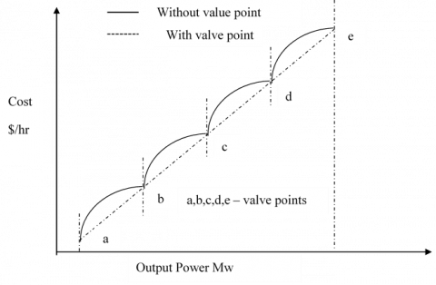
Practically viewing, owing to the presence of valve point effects, the actual characteristics are non-linear and the fuel equation becomes a non-smooth equation. These fuel curve discontinuities are caused by the actions of the valve points. The fuel equation because of the non-linear characteristic includes rectified sinusoidal term to include effect in the actual fitness function. Figure 1 shows the fuel cost curve including the effect of the valve point. The effect of the valve-point is included in the fuel cost function as follows.
Figure 1. Fuel cost curve with the impact of valve point
The cost equation of each thermal plant is defined as:
${{F}_{i}}({{P}_{gi}})={{a}_{i}}{{P}_{gi}}^{2}+{{b}_{i}}{{P}_{gi}}+{{c}_{i}}$ (4)
where, ai, bi and ci represents the cost coefficients for ith generator.
The fuel cost equation including valve point effect is given by:
${{F}_{i}}({{P}_{gi}})=\sum\limits_{i=1}^{{{N}_{g}}}{{{a}_{i}}P_{gi}^{2}}+{{b}_{i}}{{P}_{gi}}+{{c}_{i}}+{{e}_{i}}\sin ({{f}_{i}}({{P}_{gi}}^{\min }-{{P}_{gi}}))$ (5)
The values ei and fi are the cost coefficients of fuel for each unit relative to the valve point. The objective function to be reduced is defined by
${{F}_{T}}=\sum\limits_{i=1}^{{{N}_{g}}}{{{a}_{i}}{{P}_{gi}}^{2}}+{{b}_{i}}{{P}_{gi}}+{{c}_{i}}+\left| {{e}_{i}}\sin ({{f}_{i}}({{P}_{gi}}^{\min }-{{P}_{gi}})) \right|$ (6)
In this section, the various naturally inspired algorithms such as particle swarm intelligence, quantum behaved particle swarm intelligence and shuffled frog leaping algorithms are discussed in detail with flowchart and algorithms. Finally, the implementation of those algorithms for economic load dispatch is explained.
3.1 Particle swarm optimization (PSO)
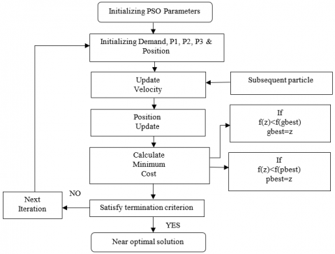
The birds are considered as particles and the concept is derived from birds or fishes; it is known as swarm intelligence technique. It is used to solving many types of power quality or power system problems. Economic dispatch is one among them which includes economic dispatch with restricted operational areas, sustainable economic dispatch and multi-area economic dispatch with tie-line restrictions. When PSO [6] is applied for all sorts of economic dispatch concepts, it gave good results when compared with lambda iteration, integer programming and genetic algorithm etc. The implementation of PSO for economic dispatch is shown in Figure 2.
Figure 2. Implementation of PSO for economic dispatch
It is a stochastic population-oriented optimization algorithm inspired by the fishes and birds searching for food. In this technique, every probable result is a point in the search space termed as ‘particle’. Each particle is having two components such as position and velocity. The velocity and position of each individual particle is denoted using the following vectors:
Vi = (Vi1, Vi2…, Vin) (7)
Xi = (Xi1, Xi2…, Xin) (8)
There are two best positions in this swarm intelligence technique. The first one is pbest which is the best solution to that particular swarm and gbest is the best solution among all the swarms. The aim of the approach is to estimate the best possible solution to the objective function. In the beginning, few particles need to be randomly generated in the search space. In each iteration, the best position of every particle will be stored which is termed as pbest and the overall best is termed as gbest. By knowing the particle's own position and the position of neighbors’, the particles or birds could reach the optimal place of solution.
INITIALIZATION OF PSO PARAMETERS:
No. of particles = 20
No. of iterations = 100
Dimension of the problem space = 3 & 13
Velocity constants C1 and C2 = 2
Inertia factor= 0.5
3.2 Quantum particle swarm optimization (QPSO)
This section deals with QPSO [7] in solving economic dispatch to find the near-optimal values of power from thermal energy systems. Quantum particle swarm intelligence is used to find the most favorable values of power from each thermal unit without violating the constraints of each unit so as to reduce the operational cost. This method is giving better results when compared with naturally inspired approaches viz. Particle swarm intelligence, Genetic algorithm, Bee colony algorithm SO and some other traditional methods like Lambda iteration method, integer programming etc.
The main difference in Quantum particle swarm intelligence is that each particle is showing quantum behavior unlike particle swarm technique and the wave function ψ(x,t) is used instead of the velocity and position components as used in particle swarm intelligence technique. Since the consequence of wave function is high, the location of the particle will be determined using the function called probability density is given by ǀψ(x,t)ǀ. With this Monte Carlo method used in the quantum particle swarm optimization technique, the location of the particle during each iteration can be evaluated using the equation below (9).
$z_{ij}^{n+1}=q_{ij}^{n}\pm \alpha .H_{ij}^{n}.ln(1/v_{ij}^{n})$ (9)
where, vijt is a random number distributed equally between (0,1) and $q_{ij}^{n}$ is a local attractor defined as:
$q_{ij}^{n}=\Phi _{ij}^{n}.q_{ij}^{i}+(1-\Phi _{ij}^{n}).q_{gj}^{n}$ (10)
where, $\Phi _{ij}^{n}$ is a random number that is equally distributed between (0,1) and the $H_{ij}^{n}$ is calculated by:
$H_{ij}^{n}=2\cdot \alpha \cdot \left| q_{ij}^{n}-z_{ij}^{n} \right|$ (11)
where, the term α represents Contraction-Expansion (CE) coefficient, used to fine-tune the convergence rate of the technique. Then the position updated by equation:
$z_{ij}^{n+1}=q_{ij}^{n}\pm \alpha \cdot \left| q_{ij}^{n}-z_{ij}^{n} \right|\cdot \ln (1/v_{ij}^{n})$ (12)
The center of all the personal best pbest positions of the total swarm is called as mbest which is given by:
$mbes{{t}^{n}}=\left( \frac{1}{K}\sum\limits_{i=1}^{K}{q_{i1}^{n},}\frac{1}{K}\sum\limits_{i=1}^{K}{q_{i2}^{n},...\frac{1}{K}\sum\limits_{i=1}^{K}{q_{ij}^{n},}...\frac{1}{K}\sum\limits_{i=1}^{K}{q_{iD}^{n}}} \right)$ (13)
where, the population size is K and the personal best position is given by qi. The term L is defined by:
$L_{ij}^{n}=2\cdot \alpha \cdot \left| mbest_{j}^{n}-z_{ij}^{n} \right|$ (14)
Finally, the position of the particle is revised with the following equation:
$z_{ij}^{n+1}=q_{ij}^{n}\pm \alpha \cdot \left| mbest_{j}^{n}-z_{ij}^{n} \right|\cdot \ln (1/v_{ij}^{n})$ (15)
With the final Eq. (15), the PSO is finally called Quantum behaved swarm intelligence approach.
INITIALIZATION OF QPSO PARAMETERS:
Swarm size or No. of Particles= 50
No of iterations= 100
Dimension of the problem space= 3 & 13
The speed of convergence of the algorithm can be adjusted by adjusting the value α of the algorithm. QPSO made another innovation by introducing a new term called mbest. Every particle in the swarm will get converged to overall best without considering other particles in PSO. But in the case of QPSO, without considering the colleagues, the particles are unable to move to the overall best position is the best highlight in this approach. The distance between particles present position and mbest is used to determine the distribution of the position of each particle for the next iteration. Particles that are far from the best overall location are called lagged particles. If some of the particles are close to global best and many of the particles are located away from position global best, then the lagged particles will pull away from the mbest.
When the particles lagged moving with the colleagues converging to Pg, Pg will be approached by mbest slowly. The distance between pbest of a particle and gbest does not reduce quickly decelerating particle convergence near Pg and the global search will be done until the lagged ones are near to Pg. As a result, in the QPSO technique, the swarm never denies the lagged particle and appears more intelligent and highly cooperative compared to the PSO.
3.3 Shuffled frog leaping approach (SFLA)
SFLA [8, 9] can be applied to all types of engineering problems such as optimizing the values of the PID controller, power system problems and scheduling problems etc. The convergence speed of the algorithm which is very fast in case of shuffled frog leaping technique is a great benefit. In this approach, the frogs are split into many groups called as a memeplex. In each memeplex, there are several numbers of frogs and each frog has its individual thoughts within the memeplex.
Since there are n numbers of the memeplex, each frog will be affected by other frog ideas in the corresponding memeplex. Once the memetic evolution steps are evolved, ideas of all frogs in memeplex are passed in the shuffling process. The local search for the best value and the shuffling process will continue until the convergence criteria have been met. Convergence criteria can usually be defined as follows:
(1) The relative fitness improvement of the global frog over a number of consecutive shuffling iterations is below the pre-defined threshold.
(2) The maximum predetermined amount of shuffling iterations has been achieved.
The shuffled frog leaping algorithm introduced to solve the economic load dispatch problem is as follows:
Step[1]. Initialization of power demand, constraints, and fuel cost coefficients.
Step[2]. Initial populations of P frogs are formed at random for an S-dimensional problem.
Step[3]. Determine the fitness value i.e. fuel cost of each frog according to the predetermined equality and inequality constraints. Once determined, the best frog position will be recorded in the whole population.
Step[4]. After the fitness values are determined, the frogs have to arranged in descending order in accordance with the fuel cost which is the fitness value of our problem.
Step[5]. The entire frogs were divided into m number of memeplexes and each of which contains n frogs.
Step[6]. In every memeplex, the frogs will be calculated for best and worst values of fitness value and they are denoted as Xb and Xw respectively. The best value among the n number of memeplex based on the fitness value is called as Xg.
Step[7]. Once the fitness value is calculated for a predefined number of the memeplex, all the frogs of the corresponding memeplex will be arranged from the best value to the worst value of fitness.
Step[8]. When the fitness value fuel cost gets converged or if there is no change in the value after certain iterations, the algorithm will be terminated and the obtained results of the best fitness value will be displayed.
Step[9]. End the procedure.
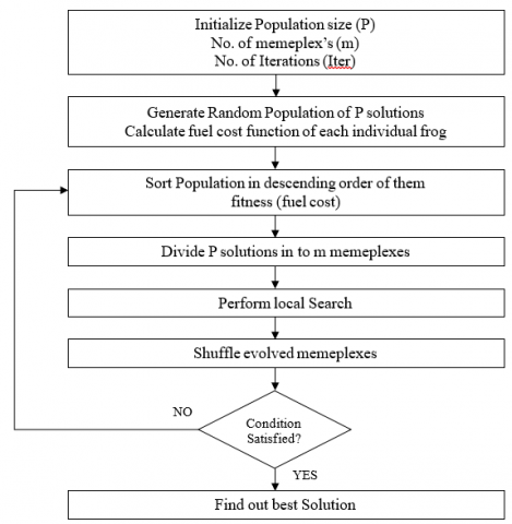
Figure 3. Implementation of SFLA for economic dispatch
If the criterion or the fitness values obtained are not satisfied, then fitness values will be calculated again and all the steps will be repeated until the near optimal value of the fuel cost are obtained. The implementation of SFLA for economic dispatch is shown in Figure 3. MATLAB execution of calculate total cost and time shown in Figure 4 and Figure 5.
INITIALIZATION OF SFLA PARAMETERS:
Total No. of Frogs= 100
No. of memeplexes= 10
No. of Dimensions= 3 & 13
No. of Iterations=50
Figure 4. MATLAB execution to calculate total cost
Figure 5. MATLAB execution to calculate time for iterations
3.4 Genetic Algorithm (GA) and Lambda Iteration (LI) method
GA is an important optimization technique for which the expected solution is to be the global solution [10]. Genetic algorithms are a class of stochastic search algorithms that begin with a population of randomly generated candidates and 'evolve' towards better solutions by applying operators-mutation, crossover, and reproduction based on genetic processes occurring in nature. GAs is naturally suited for the solution of maximization problems. Minimization problems are first converted into appropriate maximization problems for fitness functions. Genetic algorithm performance is mainly controlled by the probability of crossover and mutation. Depending on the problem, we have to select the values of these probabilities, and selecting the appropriate values of those probabilities becomes an optimization problem.
STEPS in GA:
STEP 1: Determine the Objective Function (OF).
STEP 2: Assign number of generations to 0 (t=0).
STEP 3: Create individuals randomly in the initial population P(t).
STEP 4: Determine individuals in population P(t) using OF.
STEP 5: While the termination criterion is not satisfied to do t=t+1.
Select the individuals to population P(t) from P(t-1) Change individuals of P(t) using crossover and mutation.
Evaluate individuals in population P(t) using OF.
End While
STEP 6: Return the best individual found during the evolution.
In the Lambda Iteration (LI) process, lambda is the vector used to solve constraint optimization problems called a Lagrange multiplier [11]. Since all of the inequality constraints are to be met in each case, iterative approach solves the equations.
The steps involved in the LI method are:
STEP 1: Assuming suitable λ value, that will be more than the largest interception of the incremental costs characteristic of the several generators.
STEP 2: Evaluate the individual generations.
STEP 3: Check the equality.
STEP 4: If not, repeat the second guess λ of the steps above.
In this paper, two case studies have been considered. (i.e) 3 generator system and 13 generator system. 3 generator systems and 13 generator systems [12] have to satisfy a load demand of 850 MW and 1800 MW respectively. The objective of this work is to find the power from individual units in such a way that the total demand should be met at minimum possible cost. For example, the power demand of 850MW or 1800 MW cam be found in different combinations of power. But the condition is that the combination of power from different units should result in minimum fuel cost.
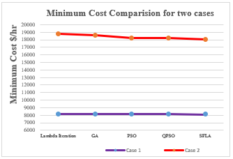
All the approaches were done for the lossless network with the valve point effect denoted by sine function in the fitness equation. The data for three generator systems and thirteen generator systems are shown in Tables 1 and 3 respectively. Similarly, the results obtained for 3 and 13 generator systems are shown in Tables 2, 4 and 5 respectively. From the result, it is observed that SFLA gives the best fuel cost and best time compared with other techniques. Figure 6 shows the minimum comparison of case 1 and case 3 for different optimization techniques.
Figure 6. Minimum cost comparision for Case 1 and Case 2
Table 1. Case 1: Data for 3 unit system
|
|
PLANT 1 |
PLANT 2 |
PLANT 3 |
|
ai ($/hr) |
0.001562 |
0.00194 |
0.00482 |
|
bi ($/Mwh) |
7.92 |
7.85 |
7.97 |
|
ci ($/Mw2h) |
561.00 |
310.00 |
78.00 |
|
ei ($/h) |
300.00 |
200.00 |
150.00 |
|
fi (1/Mw) |
0.0315 |
0.042 |
0.063 |
|
Pgimin (Mw) |
100.00 |
100.00 |
50.00 |
|
Pgimax (Mw) |
400.00 |
600.00 |
200.00 |
Table 2. Results for Case 1: 3 unit system with valve point effect
|
Approach |
P1 (mW) |
P2 (mW) |
P3 (mW) |
Best Cost ($/HR) |
Best Time (Secs) |
|
Lambda Iteration |
359 |
376 |
115 |
8269.64 |
48.70 |
|
GA |
498.54 |
252.82 |
98.63 |
8241.17 |
33.12 |
|
PSO |
300.26 |
400.00 |
149.73 |
8234.07 |
0.2887 |
|
QPSO |
320.19 |
371.10 |
158.70 |
8229.61 |
0.2641 |
|
SFLA |
320.19 |
371.10 |
158.70 |
8038.30 |
0.1572 |
Table 3. Results for Case 1: 3 unit system without valve point effect
|
Approach |
P1 (mW) |
P2 (mW) |
P3 (mW) |
Best Cost ($/HR) |
Best Time (Secs) |
|
Lambda Iteration |
394 |
335 |
121 |
8194.50 |
50.47 |
|
GA |
391.94 |
332.75 |
125.27 |
8194.48 |
20.54 |
|
PSO |
393.16 |
334.60 |
122.22 |
8194.35 |
0.3181 |
|
QPSO |
390.97 |
336.12 |
122.85 |
8194.21 |
0.2943 |
|
SFLA |
392.92 |
334.37 |
122.70 |
8194.04 |
0.1240 |
Table 4. Generator data Case 2 – 13 unit system
|
Coefficients of 3 generator System |
Pgimin (Mw) |
Pgimax (Mw) |
||||
|
ai |
bi |
ci |
ei |
fi |
||
|
0.00028 |
8.1 |
550 |
300 |
0.035 |
0 |
680 |
|
0.00056 |
8.1 |
309 |
200 |
0.042 |
0 |
360 |
|
0.00056 |
8.1 |
307 |
150 |
0.042 |
0 |
360 |
|
0.0324 |
8.74 |
240 |
150 |
0.063 |
60 |
180 |
|
0.0324 |
8.74 |
240 |
150 |
0.063 |
60 |
180 |
|
0.0324 |
8.74 |
240 |
150 |
0.063 |
60 |
180 |
|
0.0324 |
8.74 |
240 |
150 |
0.063 |
60 |
180 |
|
0.0324 |
8.74 |
240 |
150 |
0.063 |
60 |
180 |
|
0.0324 |
8.74 |
240 |
150 |
0.063 |
60 |
180 |
|
0.0284 |
8.6 |
126 |
100 |
0.084 |
40 |
120 |
|
0.0284 |
8.6 |
126 |
100 |
0.084 |
40 |
120 |
|
0.0284 |
8.6 |
126 |
100 |
0.084 |
55 |
120 |
|
0.0284 |
8.6 |
126 |
100 |
0.084 |
55 |
120 |
Table 5. Results for Case 2: 13 unit system
|
Power (MW) |
Lambda Iteration |
GA |
PSO |
QPSO |
SFLA |
|
P1 |
456.00 |
539.05 |
269.19 |
628.31 |
538.52 |
|
P2 |
257.00 |
238.03 |
360.00 |
224.39 |
74.69 |
|
P3 |
284.00 |
231.78 |
112.20 |
157.07 |
104.71 |
|
P4 |
113.00 |
98.48 |
159.66 |
109.86 |
159.70 |
|
P5 |
112.00 |
103.86 |
109.71 |
109.86 |
159.71 |
|
P6 |
66.00 |
133.29 |
60.00 |
60.00 |
159.59 |
|
P7 |
66.00 |
115.58 |
109.87 |
159.73 |
159.69 |
|
P8 |
109.00 |
96.33 |
109.87 |
60.00 |
109.86 |
|
P9 |
106..00 |
65.15 |
159.62 |
60.00 |
109.84 |
|
P10 |
72.00 |
43.85 |
119.97 |
40.00 |
40.00 |
|
P11 |
42.00 |
42.29 |
75.50 |
76.49 |
73.28 |
|
P12 |
44.00 |
45.68 |
40.00 |
40.00 |
40.00 |
|
P13 |
73.00 |
46.56 |
114.36 |
74.24 |
70.36 |
|
Min Cost ($/hr) |
18752.88 |
18606.51 |
18235.1 |
18204.2 |
18027.5 |
|
Time (secs) |
114 |
6.2198 |
1.2052 |
0.8174 |
0.2660 |
In this work, the economic aspect of the power generation system is the sole objective. Hence, we considered the maximization of profit and minimization of production costs as a priority and thus total production cost is minimized by allocating the suitable value of power from each thermal generating unit to supply the total load demand. Shuffled frog leaping algorithm is the only technique that gives better-optimized results with reduced computational time. Particle swarm optimization and quantum behaved particle swarm optimization shows less optimized results than SFLA and the values obtained from SFLA are much better than the few mentioned naturally inspired algorithms and conventional methods in terms of precision, accurate results and computational speed. The proficiency of the approach is best illustrated with the given data and proves that it is the most suitable approach for the Economic Load Dispatch problem. In future recent algorithms like BAT Algorithm, Whale Optimization Algorithm and Artificial Fish Swarm Algorithm can be used.
[1] Singal, S.K. (2007). Review of augmentation of energy needs using renewable energy sources in India. Renewable and Sustainable Energy Reviews, 11(7): 1607-1615. https://doi.org/10.1016/j.rser.2005.11.002
[2] Irfan, M., Zhao, Z.Y., Ahmad, M., Mukeshimana, M.C. (2019). Critical factors influencing wind power industry: A diamond model based study of India. Energy Reports, 5: 1222-1235. https://doi.org/10.1016/j.egyr.2019.08.068
[3] Sinha, N., Chakrabarti, R., Chattopadhyay, P.K. (2003). Evolutionary programming techniques for economic load dispatch. IEEE Transactions on Evolutionary Computation, 7(1): 83-94. https://doi.org/10.1109/TEVC.2002.806788
[4] Dike, D.O., Adinfono, M.I., Ogu, G. (2013). Economic dispatch of generated power using modified lambda-iteration method. IOSR Journal of Electrical and Electronics Engineering, 7(1): 49-54. https://doi.org/10.9790/1676-0714954
[5] Baskar, S., Subbaraj, P., Rao, M.V.C. (2003). Hybrid real coded genetic algorithm solution to economic dispatch problem. Computers & Electrical Engineering, 29(3): 407-419. https://doi.org/10.1016/S0045-7906(01)00039-8
[6] Abido, M.A. (2009). Multiobjective particle swarm optimization for environmental/economic dispatch problem. Electric Power Systems Research, 79(7): 1105-1113. https://doi.org/10.1016/j.epsr.2009.02.005
[7] Dos Santos Coelho, L. (2010). Gaussian quantum-behaved particle swarm optimization approaches for constrained engineering design problems. Expert Systems with Applications, 37(2): 1676-1683. https://doi.org/10.1016/j.eswa.2009.06.044
[8] Hasanien, H.M. (2015). Shuffled frog leaping algorithm for photovoltaic model identification. IEEE Transactions on Sustainable Energy, 6(2): 509-515. https://doi.org/10.1109/TSTE.2015.2389858
[9] Li, J., Pan, Q., Xie, S. (2012). An effective shuffled frog-leaping algorithm for multi-objective flexible job shop scheduling problems. Applied Mathematics and Computation, 218(18): 9353-9371. https://doi.org/10.1016/j.amc.2012.03.018
[10] Amjady, N., Nasiri-Rad, H. (2009). Economic dispatch using an efficient real-coded genetic algorithm. IET Generation, Transmission & Distribution, 3(3): 266-278. https://doi.org/10.1049/iet-gtd:20080469
[11] Mudumbai, R., Dasgupta, S., Cho, B.B. (2012). Distributed control for optimal economic dispatch of a network of heterogeneous power generators. IEEE Transactions on Power Systems, 27(4): 1750-1760. https://doi.org/ 10.1109/TPWRS.2012.2188048
[12] Yang, H.T., Yang, P.C., Huang, C.L. (1996). Evolutionary programming based economic dispatch for units with non-smooth fuel cost functions. IEEE transactions on Power Systems, 11(1): 112-118. https://doi.org/10.1109/59.485992