Sujuan Li
© 2020 IIETA. This article is published by IIETA and is licensed under the CC BY 4.0 license (http://creativecommons.org/licenses/by/4.0/).
OPEN ACCESS
This paper aims to design an effective scheduling method for bike sharing system that minimizes the supply-demand gap in different areas. Based on the actual data on bike sharing in a city, the spatiotemporal features of bike sharing demand were analyzed through the prediction by a backpropagation neural network (BPNN), whose structure was determined through linear regression and other techniques. According to the predicted demands, multiple assumptions and constraints were proposed for optimization of bike sharing scheduling. On this basis, a decision model for bike sharing in peak hours was established with fixed time window, with the aim to minimize the scheduling cost. Then, the genetic algorithm (GA) was improved to solve the model. Our model and the GA were proved feasible through a case analysis. This research provides a reference for optimizing the operation and management of bike sharing, and promotes the public transport in large cities.
big data analysis, decision model, bike sharing, backpropagation neural network (BPNN), linear regression
Currently, bike sharing companies are striving to establish a decision support system for their services based on big data technology. However, the application of big data analysis is bottlenecked by the inaccurate prediction of relevant data, such as the number of bikes to be rented and returned at a bike station in the next half an hour. The inaccuracy stems from the overlook of business evolution and external impacts in previous prediction methods [1-4], all of which solely depend on statistical analysis of historical data samples.
Many scholars have attempted to optimize the scheduling of bike sharing. For example, Khatri et al. [5] designed a suitable scheduling plan for bike sharing through GPS data analysis. Sun et al. [6] analyzed the use mode of bike sharing through spatiotemporal clustering, a nonlinear autoregressive neural network method, and then studied the scheduling of bike sharing. With the aid of backpropagation neural network (BPNN), Gao et al. [7] forecasted the initial scheduling of bike sharing, constructed a scheduling model to minimize the scheduling times, and obtained the optimal scheduling times by solving the model on simulation software. Kacem et al. [8] improved the single-station scheduling model for the static scheduling of bike sharing, and designed two algorithms to separately solve the scheduling model, namely, the hybrid variable neighborhood algorithm and the large neighborhood search algorithm. Li et al. [9] examined the time-varying features of scheduling benchmark threshold, bike turnover rate, and rental volume difference at bike stations, and developed a method for obtaining the dynamic scheduling time domain of bike sharing system based on self-flow model.
To effectively schedule the bike sharing system, this paper designs a decision model for bike sharing based on linear regression and the BPNN. Firstly, the bike sharing demands in different regions were predicted based on the BPNN. Next, several assumptions and constraints were proposed on the optimization of bike sharing scheduling. On this basis, an area scheduling model for rush hours was constructed with a fixed time window, aiming to minimize the scheduling cost. Then, the genetic algorithm (GA) was improved to solve the model. The effectiveness of our model and the improved GA were verified through a case analysis.
This research makes the following contributions: the proposed model helps to minimize the supply-demand gap of bikes in rush hours in different areas of the target city; the effective prediction of bike sharing demand makes it possible to analyze and forecast the rent/return behavior of each user, and to build an automatic bike supply and monitoring system; the results of spatiotemporal analysis can be fed back to bike sharing companies, providing decision support to the scheduling of bike sharing system; the research provides a reference for optimizing the operation and management of bike sharing, and promotes the public transport in large cities.
2.1 Terms and definitions
Some special terms of bike sharing are defined in Table 1.
2.2 Indices
2.2.1 Indices of launched bikes
The situation of launched bikes can be measured by the following indices:
(1) Percentage of available bikes = the number of available bikes / the number of total bikes × 100%; this index reflects the repair and maintenance ability of the bike sharing company.
(2) Percentage of launched bikes = the number of launched bikes / the number of available bikes × 100%; this index reflects the bike launch ability of the bike sharing company
(3) Percentage of unavailable launched bikes = the number of unavailable launched bikes / the number of launched bikes × 100%; this index reflects the quality of launched bikes.
(4) Percentage of long-term occupied bikes = the number of long-term occupied bikes / the number of owned bikes × 100%; this index reflects the proportion of bikes that are no longer controlled by the bike sharing company.
Table 1. Special terms of bike sharing
|
Name |
Definition |
|
Owned bikes |
The bikes owned by the bike sharing company, excluding those near the end of service life |
|
Available bikes |
The bikes that are available for sharing; other bikes are unavailable for various reasons (e.g. repair and maintenance). |
|
Launched bikes |
The bikes that are being rented, to be rented, or offline |
|
Online bikes |
The bikes that are being rented, or to be rented; other bikes are offline, which will be relaunched or remain idle. |
|
Unavailable launched bikes |
The launched bikes that cannot be rented for various reasons |
|
Long-term occupied bikes |
The bikes that have not been returned for a long time or have been removed after remaining idle for a long time |
2.2.2 Indices of bike turnover rate
(1) Single bike turnover rate = the number of rented bikes / the number of owned bikes × 100%
(2) Single bike turnover rate at station: the single bike turnover rate calculated based on the data on a station
(3) Top-k single bike turnover rates: the highest k single bike turnover rates
(4) Bottom-k single bike turnover rates: the lowest k single bike turnover rates
(5) Percentage of offline bikes = the number of offline bikes / (the number of online bikes + the number of offline bikes) × 100%; this index should be minimized to improve bike sharing.
(6) Percentage of re-launched bikes = the number of re-launched bikes / the number of offline bikes × 100%
(7) Time ratio of idle offline bikes = no bike rental period × the number of offline bikes; this index reflects the waste of resources due to no rental of online bikes and idle offline bikes
(8) Mean rental time: the mean rental time of a station; this index is negatively correlated with the bike turnover rate.
(9) Top-k single mean rental times: the highest k means rental times
(10) Bottom k means rental time: the lowest k means rental times
2.2.3 Failures of bike sharing system
(1) Time or times of the first failure (TTFF): the service time or times of the first failure of the system
(2) Mean time between failures after the first failure (MTFF): the mean time between failures after the system failed for the first time
(3) System mean repair time (SMRT): this index reflects the self-recovery ability of the system.
(4) Arrival of the MTFF limit: this index warns that the system is about to reach the MTTF.
(5) System failure time: the service time that the bikes stop service and the turnover suspends due to system failure
3.1 Data preprocessing
The research data come from the bike sharing orders of a city in China. The data were collected from the business system and management system of bike sharing companies, and the public traffic cards of the residents in the city.
The actual data can objectively reflect the spatiotemporal distribution features of bike sharing. The original data cover the following attributes: order ID, user ID, bike ID, bike type, start date of rental, rental period, start location, and end location. In total, there are includes 3,213,996 rent/return orders from May 15 to 29, 2018, involving 348,745 users and 473,798 bikes.
To eliminate the interference of weather, the samples on cloudy or sunny days with good air quality, that is, May 15 to 21, 2018, were retained for further analysis. To disclose the time distribution features, several fields were added to the selected samples, namely, date, hour, week, and workday/weekend.
3.2 Daily distribution analysis
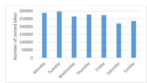
Firstly, the number of rented bikes on each day in a week was statistically analyzed.
The analysis results (Figure 1) show that the number of rented bikes on weekdays was above the daily average, while that on weekends was below the daily average. Far more bikes were rented on each weekday than on each weekend day.
Figure 1. Daily distribution of bike sharing in a week
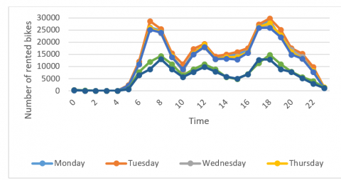
Figure 2. Hourly distribution of bike sharing in a day
3.3 Hourly distribution analysis
Next, each day in the week was evenly split into 24 periods. The number of rented bikes was calculated for each period on each day in the week to reveal the variation of bike sharing with hours.
As shown in Figure 2, the hourly distribution of bike sharing had three peaks from Monday to Friday, including 7:00-8:00 in the morning, 11:00-12:00 at noon, and 17:00-18:00 in the evening. The morning and evening peaks were much higher than the noon peak and the other segments of the hourly distribution curves. This is because commuters are the leading bike sharers on workdays. The number of rented bikes is maximized in the morning and evening rush hours. During the lunch hours, some commuters rent bikes to visit restaurants or canteens, resulting in a rise of short-distance ridings.
By contrast, the hourly distribution of bike sharing on weekends was relatively balanced, without any obvious peaks in the morning, at noon, or in the evening.
3.4 Typical day analysis
Through the above analysis, it is learned that lots of bikes were rented on May 17. Hence, the geographical coordinates of the start locations in the morning peak and those of the end locations in the evening peak were analyzed based on the data on May 17.
The analysis shows that, in the early peak, most rented bikes ended at rail transit stations; in the evening peak, most rented bikes left from rail transit stations. Overall, the density of rented bikes peaked around rail transit stations, and gradually decreased with the distance away from these stations. This confirms that most bikes are rented by commuters in the morning and evening rush hours on workdays.
To ease the uneven distribution of rented bikes and rationalize the scheduling of bike sharing, this section sets up a BPNN-based demand prediction model after analyzing the bike sharing demand in each region and each period.
4.1 Input and output variables
In the BPNN, the number of input layer nodes depends on the dimensions of input data, while the number of output layer nodes depends on the objective of the problem. In our problem, the objective is to predict the bike sharing demand in each period. This was taken as the output variable of the BPNN. Meanwhile, input variables of the BPNN were determined through linear regression [10, 11].
According to the big data analysis in Section 3, weekdays and weekends differed greatly in the distribution of bike sharing, while the weekdays were similar in hourly distribution of bike sharing. Here, linear regression is performed to identify the factors highly correlated with the bike sharing demand in the current and future periods. These factors were taken as the input variables of the BPNN, laying the basis for predicting the demand in different periods of future.
The samples were collected from 5:00-23:00, because the number of rented bikes was low before 5:00 and after 23:00 on workdays. First, the hourly demands in 5:00-23:00 were taken from the same area on each day, and subjected to linear regression. The results show that hourly demands were not significantly correlated. The highest degree of correlation was below 0.9. Negative correlations were observed in some cases. Therefore, the hourly number of rented bikes on the same day was not regarded as an input variable of the BPNN.
Similarly, the daily demands were also subjected to linear regression, revealing the strong correlations between daily demands. As a result, the historical data on similar days were inputted to the BPNN to forecast the bike sharing demand on the future day.
4.2 Datasets and learning rate
To predict the bike sharing demand in different areas, the BPNN [12, 13] should be provided with the historical data on bike sharing demand in each forecast area. These data were divided into a training set, a validation set, and a test set. As its name suggests, the training set is used to train the BPNN. The trained model will be verified on the validation set. If the error falls within the preset interval, the trained BPNN will be applied to predict the bike sharing demand on the test set. The prediction results will be inversely normalized to obtain the predicted number of rented bikes. If the error falls outside the preset interval, the BPNN will be trained again with more iterations, until the error on the validation set falls within that interval.
The learning rate has a greatly impact on the training effect [14]. If it is too small, the training will be slow; if it is too large, the training error will exceed the minimum value, despite a rapid decline in the initial phase of training. In the latter case, it is difficult and even impossible for the BPNN to converge to the optimal solution. Here, the learning rate is empirically selected from the interval of 0.01-0.8, and used to train the BPNN repeatedly. The decline rate of the error sum of squares (ESS) was observed after each training. In this way, the optimal learning rate was determined as 0.001. Similarly, the maximum number of iterations was set to 6,000, while the weights and thresholds were initialized randomly.
4.3 Number of hidden layer nodes
The typical structure of the BPNN includes an input layer, a hidden layer, and an output layer. Each layer has a certain number of nodes [15]. This structure was adopted for our research, for one hidden layer is sufficient to realize all kinds of nonlinear mappings. The number of input and output layer nodes, i.e. the number of input and output variables, was determined in the preceding subsections. Thus, this subsection aims to select the optimal number of hidden layer nodes.
At present, there is no definite formula to determine the number of hidden layer nodes. The traditional empirical approach merely gives the optimal range of that number, and narrows down the range through repeated trainings of the prediction model. The empirical formula [16, 17] for calculating the interval can be expressed as:
$m=\sqrt{n_{i}+n_{o}}+a$ (1)
where, ni and no are the number of input and output layer nodes, respectively; a∈[1, 10] is a constant.
By formula (1), the optimal range of the number of hidden layer nodes was narrowed down to [6, 12]. Then, the BPNN was trained repeatedly with 5 hidden layer nodes at first. The number of hidden layer nodes was increased by 1 in each additional training until reaching 12. Through the trainings, the prediction error was minimized and the model converged at the fastest rate, when there were 10 hidden layer nodes. As a result, 10 was selected as the optimal number of hidden layer nodes.
4.4 Example analysis
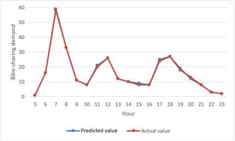
Figure 3. Comparison between predicted demand and actual demand
The BPNN was trained by the bike sharing demands in the area of a station on 9 workdays from May 15 to May 28, 2018, and then used to predict the hourly demand on May 24 in the same area. Figure 3 compares the predicted demand with the actual demand. Obviously, the time-varying trend of the predicted demand was close to that of the actual demand, indicating that the trained BPNN has good prediction accuracy.
Over the time, the rented bikes are rode to different areas. The number of bikes entering or leaving an area varies from place to place. This leads to the imbalance of bike supply and demand in many areas. The supply-demand gap must be bridged through proper scheduling of the bike sharing system.
According to the above analysis, in terms of time, the bike sharing demand concentrated in morning and evening rush hours on workdays; in terms of space, the rented bikes clustered in hotspots, i.e. rail transit stations, during the morning and evening rush hours. Therefore, the scheduling of bike sharing in an area should focus on the rush hours in the hotspots, when there is a large demand for bike sharing.
5.1 Area scheduling model
The scheduling of bike sharing is a complex, systematic problem, involving multiple variables and constraints [18]. To ensure the feasibility and explanatory power of our model, the following assumptions were made prior to modelling:
(1) There is only one station in the area, which sends/collects bikes to/from multiple hot spots. The station has enough bikes to meet the needs of all hotspots.
(2) The geographical coordinates of the station and each hotspot are known, so is the distance between the station and each hotspot. The effects of external factors like weather and traffic conditions on the scheduling process are not considered.
(3) The scheduling demand of each hotspot in the current cycle is known and stable.
(4) The bikes to be sent/collected to/from a hotspot are transported by a vehicle at only one time.
(5) The vehicle only passes through the target hotspot once.
(6) The damage and maintenance of the vehicle are not considered.
(7) The bike supply and demand are balanced in all hotspots at the start of the scheduling cycle.
Under the above assumptions and with a fixed time window, the area scheduling model for rush hours was constructed to minimize the scheduling cost:
$\begin{aligned} \min F=C_{1} \times N_{c} &+C_{0} \sum_{i=1}^{M} \sum_{j=1}^{M} \sum_{c=1}^{C} x_{i j c} \times d_{i j} \\ &+C_{2} \\ & \times \sum_{c=1}^{C} \max \left\{\sum_{i=1}^{M} \sum_{i=1}^{M} x_{i j c}\right.\\ &\left.\times\left(t_{i j c}+s_{i c}+s_{i c}\right)-1 | 0\right\} \end{aligned}$ (2)
where, Nc is the number of vehicles required for scheduling; C0 is the travel cost per unit distance; C1 is the fixed cost; C2 is the penalty cost; xijc is a binary variable (if vehicle c completes the task from hotspot i to hotspot j, xijc=1; otherwise, xijc=0); tijc is the travel time of vehicle c from hotspot i to hotspot j; sic and sjc are the service times of vehicle c in hotspot i to hotspot j, respectively.
The objective function aims to minimize the total scheduling cost, which covers the fixed cost, the travel cost, and the penalty cost of each vehicle. Specifically, the fixed cost refers to the fixed scheduling cost of each vehicle; the total fixed cost is proportional to the number of vehicles. The travel cost refers to the cost incurred by all vehicles in the area, which is proportional to the total travel distance. The penalty cost refers to the penalty imposed on a vehicle that fails to complete the task in the time window (1h). No penalty cost will be incurred if the task is completed within 1h. The above model faces the following constraints:
$0 \leq R_{i c} \leq P$ (3)
$\sum_{c=1}^{C} \gamma_{i c}=1$ (4)
$\sum_{i=1}^{M} \sum_{j=1}^{M} x_{i j c} \times d_{i j} \leq D_{c}$ (5)
$x_{i j c}, \gamma_{i c} \in\{0,1\}$ (6)
5.2 Model solving
Considering the conditions of area scheduling of bike sharing, the traditional GA was improved to solve the above model. The solving process can be broken down into six steps:
Step 1. Coding
The station in the area was given the number of 0, and the n hotspots to be served by the vehicles were numbered in turn as 1, 2, …, n. Then, the path of each vehicle could be expressed based on these serial numbers. If a vehicle leaves from the station, serves hotspots 2, 4 and 5 in turn, and then returns to the station, then the path of the vehicle can be encoded as 0, 2, 4, 5, 0.
Step 2. Population initialization
The population was initialized by random. The population size, i.e., the number of individuals in the population, was designed empirically. Then, the population size was modified repeatedly through model simulation. The size (200) that led to the best simulation effect was taken as the optimal population size.
Step 3. Fitness calculation
The fitness of each individual was calculated by:
$f i t\left(x_{i}\right)=1 /\left(f\left(x_{i}\right)+f(x)_{\min }+1\right)$ (7)
where, f(xi) is the objective function value of an individual; f(x)min is the global minimum of f(xi) in the population.
Step 4. Selection
The individuals were chosen by roulette selection, that is, an individual with a high fitness is more likely to be selected. Let N be the number of individuals in the population. Then, the selection probability of individual i can be derived from the fitness function:
$P_{i}=f i t\left(x_{i}\right) / \sum_{i=1}^{N} f i t\left(x_{i}\right)$ (8)
Step 5. Crossover
The individuals were subjected to sequential crossover at the probability of 0.8. The genes at a few randomly selected positions of parent chromosome A were copied to the same positions of child chromosome A. Then, the genes at the other positions of parent chromosome B were copied to the other positions of child chromosome A. The child chromosome B was obtained in a similar manner.
Step 6. Mutation
Mutation aims to maintain the diversity of the population, and ensure the local search ability of the algorithm. Here, the individuals are subjected to reverse mutation at the probability of 0.1.
5.3 Experimental analysis
To verify their effectiveness, the decision model and the improved GA were applied to schedule the bike sharing system in a city in China. The MATLAB was adopted as the simulation platform.
The original data were collected on May 17 in that city. The samples in the morning peak (7:00-8:00) were selected for modelling, and the entire city was divided into 22 areas. Then, the BPNN model was employed to predict the bike sharing demand of each area the scheduling cycle. The results are listed in Table 2 below.
Table 2. The predicted bike sharing demand of each area
|
Hotspot |
Demand heat |
Demand |
Meaning |
|
1 |
0.12% |
-22 |
Collection |
|
2 |
0.15% |
8 |
Sending |
|
3 |
0.13% |
14 |
Sending |
|
4 |
0.21% |
41 |
Sending |
|
5 |
0.18% |
28 |
Sending |
|
6 |
0.16% |
-9 |
Collection |
|
7 |
0.17% |
15 |
Sending |
|
8 |
0.19% |
62 |
Sending |
|
9 |
0.22% |
35 |
Sending |
|
10 |
0.14% |
-16 |
Collection |
|
11 |
0.15% |
-4 |
Collection |
|
12 |
0.20% |
-5 |
Collection |
|
13 |
0.15% |
18 |
Sending |
|
14 |
0.14% |
59 |
Sending |
|
15 |
0.12% |
-8 |
Collection |
|
16 |
0.19% |
-31 |
Collection |
|
16 |
0.11% |
46 |
Sending |
|
18 |
0.19% |
40 |
Sending |
|
19 |
0.22% |
38 |
Sending |
|
20 |
0.20% |
16 |
Sending |
|
21 |
0.19% |
-9 |
Collection |
|
22 |
0.16% |
-3 |
Collection |
To solve the decision model, a station was set up at the center of each area. Each vehicle must leave from the station half-loaded with bikes, visit each hotspot to be served, and then return to the station. On the return journey, the vehicle should not be overloaded.
According to field survey and relevant research [19, 20], the parameters of the decision model were empirically configured as shown in Table 3.
The proposed decision model was solved separately by the traditional GA and the improved GA. During solving process of the traditional GA, the optimization objective stabilized after 1,300 iterations; During the solving process of the improved GA, the optimization objective stabilized after 750 iterations, that is, the optimization speed increased by almost 40%. In addition, the improved GA reduced the scheduling cost by 9.2% from the level of the traditional GA. Overall, the improved GA outperformed the traditional GA in optimization ability and efficiency. Therefore, our decision model, coupled with the improved GA, can effectively optimize the scheduling of bike sharing system.
Table 3. Parameter values
|
Symbol |
Value |
Meaning |
|
P |
200 |
Each vehicle can carry up to 200 bikes. |
|
Dc |
150 |
Each vehicle can travel 150 km in a scheduling cycle. |
|
C0 |
10 |
Each vehicle costs RMB 10 yuan per unit distance. |
|
C1 |
80 |
The fixed cost of each vehicle is RMB 80 yuan. |
|
C2 |
200 |
If a vehicle fails to complete the task within the current cycle, it will be fined RMB 200 yuan. |
This paper mainly targets the decision-making in the scheduling of bike sharing system. Based on actual bike sharing orders, the spatiotemporal distribution features of rented bikes were analyzed visually. On this basis, the bike sharing demands in different areas were predicted with the aid of the BPNN. Then, an area scheduling model was established to optimize the scheduling of bike sharing system, and the GA was improved to solve the established model. Our model and the improved GA were proved feasible through a case study on bike sharing scheduling in a city of China. The research provides a desirable way to eliminate the supply-demand gap of bike sharing in urban areas.
[1] Levy, N., Golani, C., Ben-Elia, E. (2019). An exploratory study of spatial patterns of cycling in Tel Aviv using passively generated bike-sharing data. Journal of Transport Geography, 76: 325-334. https://doi.org/10.1016/j.jtrangeo.2017.10.005
[2] Loidl, M., Witzmann-Müller, U., Zagel, B. (2019). A spatial framework for Planning station-based bike sharing systems. European Transport Research Review, 11(1): 9. https://doi.org/10.1186/s12544-019-0347-7
[3] Park, C., Sohn, S.Y. (2017). An optimization approach for the placement of bicycle-sharing stations to reduce short car trips: An application to the city of Seoul. Transportation Research Part A: Policy and Practice, 105: 154-166. https://doi.org/10.1016/j.tra.2017.08.019
[4] Wang, X., Yang, L.T., Liu, H., Deen, M.J. (2017). A big data-as-a-service framework: State-of-the-art and perspectives. IEEE Transactions on Big Data, 4(3): 325-340. https://doi.org/10.1109/TBDATA.2017.2757942
[5] Khatri, R., Cherry, C.R., Nambisan, S.S., Han, L.D. (2016). Modeling route choice of utilitarian bikeshare users with GPS data. Transportation research record, 2587(1): 141-149. https://doi.org/10.3141/2587-17
[6] Sun, G., Bin, S. (2017). Router-Level Internet Topology Evolution Model based on Multi-Subnet Composited Complex Network Model. Journal of Internet Technology, 18(6): 1275-1283.
[7] Gao, X., Lee, G.M. (2019). Moment-based rental prediction for bicycle-sharing transportation systems using a hybrid genetic algorithm and machine learning. Computers & Industrial Engineering, 128: 60-69. https://doi.org/10.1016/j.cie.2018.12.023
[8] Kacem, I., Kadri, A., Laroche, P. (2018). A clustering-based approach for balancing and scheduling bicycle-sharing systems. Intelligent Automation and Soft Computing, 24(2): 421-430.
[9] Li, M., Liao, R., Dong, Y. (2018). A new BP neural network model for the prediction problem of equally spaced time sequences and its application. NeuroQuantology, 16(6): 28-32. https://doi.org/10.14704/nq.2018.16.6.1585
[10] Park, Y., Akar, G. (2019). Why do bicyclists take detours? A multilevel regression model using smartphone GPS data. Journal of Transport Geography, 74: 191-200. https://doi.org/10.1016/j.jtrangeo.2018.11.013
[11] Huang, P., Li, T., Shu, Z., Gao, G., Yang, G., Qian, C. (2018). Locality-regularized linear regression discriminant analysis for feature extraction. Information Sciences, 429: 164-176. https://doi.org/10.1016/j.ins.2017.11.001
[12] Abedinia, O., Amjady, N., Ghadimi, N. (2018). Solar energy forecasting based on hybrid neural network and improved metaheuristic algorithm. Computational Intelligence, 34(1): 241-260. https://doi.org/10.1111/coin.12145
[13] Chen, Y. (2018). Prediction algorithm of PM2.5 mass concentration based on adaptive BP neural network. Computing, 100(8): 825-838. https://doi.org/10.1007/s00607-018-0628-3
[14] Yu, F., Xu, X. (2014). A short-term load forecasting model of natural gas based on optimized genetic algorithm and improved BP neural network. Applied Energy, 134: 102-113. https://doi.org/10.1016/j.apenergy.2014.07.104
[15] Yu, S., Zhu, K., Gao, S. (2009). A hybrid MPSO-BP structure adaptive algorithm for RBFNs. Neural Computing and Applications, 18(7): 769-779. https://doi.org/10.1007/s00521-008-0214-2
[16] Jiang, N., Zhao, Z., Ren, L. (2003). Design of structural modular neural networks with genetic algorithm. Advances in Engineering Software, 34(1): 17-24. https://doi.org/10.1016/S0965-9978(02)00107-2
[17] Wu, W., Wang, J., Cheng, M., Li, Z. (2011). Convergence analysis of online gradient method for BP neural networks. Neural Networks, 24(1): 91-98. https://doi.org/10.1016/j.neunet.2010.09.007
[18] Ma, X., Zhang, X., Li, X., Wang, X., Zhao, X. (2019). Impacts of free-floating bikesharing system on public transit ridership, Transportation Research Part D: Transport and Environment, 76, 100-110. https://doi.org/10.1016/j.trd.2019.09.014
[19] Shivani, S., Tiwari, S. (2019). Simulation of intelligent target hitting in obstructed path using physical body animation and genetic algorithm. Multimedia Tools and Applications, 78(8): 9763-9790. https://doi.org/10.1007/s11042-018-6575-3
[20] Grzybowska, H., Kerferd, B., Gretton, C., Waller, S.T. (2020). A simulation-optimisation genetic algorithm approach to product allocation in vending machine systems. Expert Systems with Applications, 145: 113110. https://doi.org/10.1016/j.eswa.2019.113110