Arezki Adjati* | Toufik Rekioua | Djamila Rekioua
© 2020 IIETA. This article is published by IIETA and is licensed under the CC BY 4.0 license (http://creativecommons.org/licenses/by/4.0/).
OPEN ACCESS
Previously, a particular interest is focused on embedded systems and isolated sites, given that troubleshooting is not obvious in the short time. Currently, after the onset of the COVID 19 pandemic and due to the confinement imposed on almost all the countries of the world, immediate or timely repair may be impossible.
Reason why, this document provides for the study of the behavior of a pumping system, having to fill a water tower with a capacity of 150 m3 with a TDH of 17 m, during the loss of a phase, two phases or even three phases of feeding, in order to ensure control of the process and guarantee continuity of service, especially in these periods when hygiene and cleanliness are required to minimize the risk of contamination.
The results obtained show that the DSIM can still rotate even in the event of loss of supply phases or short circuit in the stator windings and provide the torque necessary to pump water under degraded conditions and after this analysis, it turns out that thanks to its flexibility and its operation in degraded mode, the DSIM will be widely used.
The global system is dimensioned and simulated under Matlab/Simulink Package.
centrifugal pump, degraded mode, dual stator induction motor (DSIM), inverters, phase opening.
The history of fault diagnosis and protection goes back to the origin of the machines themselves. Users of electrical machines initially implemented simple protection, for example against over currents, over voltage and earth fault protection, to ensure safe and reliable operation.
However, the rotation system is not immune to failure in some applications where it has now become very important to diagnose faults from their birth, because a failure in one of the constituent parts of the machine can stop the entire pumping process, causing either obvious financial loss or imminent danger [1].
In the current context of the Covid 19 pandemic, it is easy to assimilate the case of an isolated site or an on-board system with any installation, from the point of view of the impossibility of repairing breakdowns immediately. Indeed, the confinement imposed by almost all the countries in the world makes repairing breakdowns, on time, very delicate, added to this the need for this vital liquid in the almost permanent toilet to avoid the contagiousness of this virus.
It is for this reason that it is important to take an interest in the functioning of the DSIM in the presence of an anomaly in order to remedy the fault and ensure continuity of service and the most satisfactory operation possible in order to pump this precious liquid.
Mecrow et al. [2] indicates that faults in control and power converters are among the highest probabilities of drive failure with the risk of short circuit or opening of a switch. Shamsi-Nejad [3] highlights a power supply and control strategy in degraded mode during an IGBT short-circuit by short-circuiting the defective star and continuing to control the torque with the healthy inverter.
Bellara et al. [4] propose a dimensioning of an MSAP-DE tolerant to the short-circuit fault of an IGBT and have used the finite element method and have shown that the short-circuit currents can be limited.
On the other hand – Moraes et al. [5] approached the analysis of the performance of the drive in the case of a short-circuit fault of a transistor based on the modification of the control algorithm in the context of a command in degraded mode of a drive comprising two machines connected in series and controlled independently.
In this paper, we will plan to connect the neutral of the two stars in the event of failure of one phase, two phases or three phases, either of the same star or of different stars. Through this study, we will make a synthesis of the various breakdowns which can occur in the pumping chain and we will try to limit the ripples of the couple.
When, for any reason, the operation is changed at the level of the actuator or its supply by the opening of one of the phases, the operation of the system is no longer satisfactory. This mode of operation is called "degraded mode", which is none other than an exceptional operation in which one or more elements of the drive system are malfunctioning [6, 7].
If the measurements are not taken, the rotation may not be ensured and torque oscillations appear. If they are, most of the time, simply embarrassing, they are sometimes detrimental to sensitive and embarked systems.
Studies have shown that in case of opening of a stator phase, the more the machine has phases, the less the disturbance on the torque is important and that the corrugations generated increase with the number of defective phases [7].
For engines with five to nine phases, processing a phase opening follows two main strategies, either by acting on a single phase still healthy for each open phase, or by acting on each of the currents in the still healthy phases [8].
2.1 Description of a pump chain
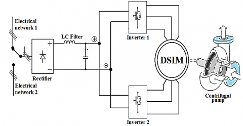
Figure 1 represents a pumping chain supplied, generally, by a main source of three-phase currents and by another backup source.
The rectifier is used to obtain a continuous bus to supply two inverters in order to obtain a double three-phase supply offset by π/6 between the stars. The DSIM is thus supplied and its shaft rotates the axis of the centrifugal pump.
Figure 1. Representation of a pumping energy chain
2.2 Causes of degraded mode
The causes of a malfunction of an energy chain are multiple and can be grouped according to the part reached by the degradation [7].
2.2.1 Network degradation
To ensure continuity of service, two three-phase networks are available at the pumping site. In the event of a main network interruption, it is possible to supply this actuator with an auxiliary network [9].
2.2.2 Degradation at the level of engine
The motor can have anomalies such as the destruction of a winding of a stator phase, a detachment of a rotor magnet, an inter-turns short circuit which can worsen and evolve towards a phase-phase short circuit or phase-to-earth, or a broken bar, a rupture of the ring, a short-circuit in the rotor windings, a ball bearing problem, rotor eccentricity, etc. [10, 11].
2.2.3 Degradation at the level of connectors
Connection includes all the techniques related to physical connections of electrical connections. The industrial connector has the distinction of being extremely robust and tolerating high voltages and constraints. The faults related to the connections can be a contact loose, a protection fuse, etc. [12].
2.2.4 Degradation at the level machine power supply
This degradation corresponds to the faults which can occur on the link and on the inverters which supply the six windings of the two stators of the machine inducing the opening of a stator supply phase and leading to the cancellation of the current.
The power transistors making up the voltage inverter may have malfunctions. These anomalies can result from normal wear and tear, improper design, improper assembly or misalignment, improper use, or a combination of these different causes [7].
The consequences of a fault generate that the voltage across a phase becomes uncontrollable and the couple will be directly infected by disturbing ripples causing annoying vibrations of the machine and annoying sound effects. The currents in the remaining windings of the machine can reach destructive values [7, 13].
In this study, the faults boil down to losses of DSIM supply phases.
2.3 Study of eventual defect
The different statistical studies on the degradation of a power supply chain show that the faults at the level of the voltage inverters and their controls are the most frequent. It is therefore justified to limit the study to failures that may occur on the power transistors, on the connectors and on the protection fuses and we will focus on the degradation of the power supply of the machine which corresponds to the defects that may occur on the link and the inverters inducing the opening of a phase of stator power supply and leading to the cancellation of the current [6, 7, 13, 14].
2.3.1 Power transistor opening defect
If one of the transistors of the inverter is in opening defect while the control of the complementary transistor is active, the short circuit of the DC power supply is inevitable and to avoid this kind of inconvenience, it is imperative to act either by canceling the control of the other transistor, or by using a fuse protection whose fusion is ultra-fast [6, 7, 13, 15].
2.3.2 Power transistor closing defect or fusing a fuse
Similarly, for this case, the voltage across the phase connected to the faulty arm becomes uncontrollable. Depending on the faulty transistor and the position of the fuse, the phase connected to the faulting arm is connected to a potential of the supply either directly or via a diode [6].
2.4 Defect isolation method
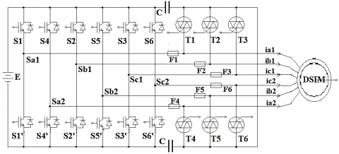
Figure 2 shows the arrangement of the triacs and the fuses used to isolate the defective phases in order to avoid passing on the problems to other organs of the energy chain. A static switch sets the voltage of the open phase to half of the DC bus voltage [16].
Figure 2. Disconnection of defective phases by the Triacs
The Table 1 associates each star phase with the corresponding IGBTs. According to Figure 2, when one of the arms of the two inverters is defective, the Triac becomes conductive and the fuse placed in series is then connected between a potential difference generating its melting and the disconnection of the phase in question. To ensure phases insulation presenting anomalies, it is necessary to use as many Triacs as phases, reason for which the control circuit is congested [7, 13].
Table 1. IGBT corresponding to the phases
|
|
First star |
Second star |
||||
|
Phases |
Sa1 |
Sb1 |
Sc1 |
Sa2 |
Sb2 |
Sc2 |
|
Associated IGBT |
S1-S1’ |
S2-S2’ |
S3-S3’ |
S4-S4’ |
S5-S5’ |
S6-S6’ |
Parallel redundancy at the power supply of the engine allows degraded operation even if a power phase is open.
2.5 Control strategy in degraded mode
The control techniques are based on the modification of the current in one or more phases to maintain a constant torque during degraded mode operation [7, 17].
Two methods exist, either by acting on the current of a single phase still healthy for each open phase, or by acting on each of the currents in the phases not in default [18].
To avoid infecting the performance of the machine which exhibits torque oscillations during a fault, the application of the two methods has the main aim of reducing these oscillations as much as possible in order to allow the most satisfactory operation possible [13].
2.5.1 Action on the current of a single phase still healthy by each open phase
When disconnecting from a faulty phase, the choice is made for a healthy phase located at 90° electrical thereof where the current is changed to ensure constant, maximum torque and limited joule losses [19].
A valid method for machines with any electromotive forces, but for machines with sinusoidal fems, the stresses of the current are concentrated on few healthy phases from where the limitation to half the number of phases.
For example, by applying this method where the Sa1 phase is open, the choice will be made for the Sb1 phase which will bear all the stress of the fault, hence [13]:
$i_{a 2}=I_{\max } \sin (\omega \cdot t-\pi / 6)$
$i_{b 1}=2 . I_{\max } \cos (2 \pi / 3) \sin (\omega . t)=-I_{\max } \sin (\omega . t)$
$i_{b 2}=I_{\max } \sin (\omega t-5 \pi / 6)$ (1)
$i_{c 1}=I_{\max } \sin (\omega \cdot t-4 \pi / 3)$
$i_{c 2}=I_{\max } \sin (\omega . t-3 \pi / 2)$
2.5.2 Action on each of the currents in the still healthy phases
In the case of machines with sinusoidal fems, a correction of the remaining currents by an analytical evaluation makes it possible to restore a constant torque while minimizing the joule losses [18].
The advantage lies in the fact that the degradation is distributed over the rest of the healthy phases of the machine. This method is valid as long as there are a sufficient number of phases to produce a rotating field.
For example, the application of this second method where the Sa1 phase is open, the stress is supported by all the healthy phases and, after calculation, the new setpoints of the currents will be [6]:
$i_{a 2}=1.27 I_{\max } \sin (\omega t-\pi / 3)$
$i_{b 1}=1.27 I_{\max } \sin (\omega . t-5 \pi / 6)$
$i_{b 2}=1.27 I_{\max } \sin (\omega . t-\pi)$ (2)
$i_{c 1}=1.27 I_{\max } \sin (\omega t+5 \pi / 6)$
$i_{c 2}=1.27 I_{\max } \sin (\omega t+\pi / 3)$
Even if the two methods make it possible to maintain a constant torque when disconnecting one or more phases of a machine having more than three phases, some disadvantages may be mentioned, such as the need to change the current setpoint in one or more phases. It is therefore necessary to have a system capable of detecting defecting phases in order to be able to apply the new setpoints of the current.
A table summarizing the setpoints of the current as a function of the disconnected phases is necessary [13, 20].
3.1 Centrifugal pump
The centrifugal pump is a flow generator that ensures the movement of a fluid from one point to another, when gravity does not perform this task.
BRAUNSTEIN and KORNFELD introduced in 1981 the expressions of mechanical power [21].
$P_{m e c}=K_{r} \omega_{r}^{3}$ (3)
The centrifugal pump opposes a resistant torque from which its expression is given by:
$T_{r}=K_{r} \omega_{r}^{2}+T_{s}$ (4)
The model used is identified by the expression of the TDH given by the PELEIDER-PETERMAN model [22]:
$T_{r}=K_{r} \omega_{r}^{2}+T_{s}$ (5)
where, Kr: Proportionality coefficient, ωr: rotation speed, Q: Flow and K0, K1, K2: Pump constant.
3.2 Transformation matrix
The magnetomotive force produced by the stator phases is equivalent to that produced by two quadrature windings αβ crossed by the currents isα and isβ such that:
$\left[\begin{array}{c}i_{s \alpha} \\ i_{s \beta}\end{array}\right]=\left[\begin{array}{lllllll}T c & & i & i_{a 1} & i_{a 2} & i_{b 1} & i_{b 2} & i_{c 1} & i_{c 2}\end{array}\right]^{t}$ (6)
Mathematically, a six-dimensional system cannot be reduced to a two-dimensional system. It is for this reason that, four vectors named [Z1], [Z2], [Z3] and [Z4] orthogonal to each other and orthogonal to the vectors, along the axis “α” and the axis “β”, are needed to complete the transformation.
3.3 Voltage equations
The electrical equations governing the DSIM in the reference αβ are given by [13]:
$\left\{\begin{array}{c}v_{\alpha}=R_{s} i_{s \alpha}+\frac{d}{d t} \phi_{s \alpha} \\ 0=R_{r} i_{r \alpha}+\frac{d}{d t} \varphi_{r \alpha}+\omega_{r} \phi_{r \beta} \\ v_{\beta}=R_{s} i_{s \beta}+\frac{d}{d t} \phi_{s \beta} \\ 0=R_{r} i_{r \beta}+\frac{d}{d t} \varphi_{r \beta}-\omega_{r} \phi_{r \alpha}\end{array}\right.$ (7)
3.4 Magnetic flux equations
On the other hand, the stator and rotor fluxes equations are [13, 23]:
$\left\{\begin{array}{l}\left(\begin{array}{c}\phi_{s \alpha} \\ \phi_{r \alpha}\end{array}\right)=\left(\begin{array}{cc}L_{s d} & M_{d} \\ M_{d} & L_{r}\end{array}\right)\left(\begin{array}{c}i_{s \alpha} \\ i_{r \alpha}\end{array}\right) \\ \left(\begin{array}{c}\phi_{s \beta} \\ \phi_{r \beta}\end{array}\right)=\left(\begin{array}{cc}L_{s q} & M_{q} \\ M_{q} & L_{r}\end{array}\right)\left(\begin{array}{c}i_{s \beta} \\ i_{r \beta}\end{array}\right)\end{array}\right.$ (8)
3.5 Voltage equation in space Z
In healthy operation, there are four voltages in Z space and this number of equations decreases by one unit each time an inverter arm is faulty. With ‘k=2’, ‘k=3’ or ‘k=4’, the voltage equations in Z space are:
$v_{Z_{1}}=R_{s} i_{z_{1}}+L_{1 s} \frac{d i_{z_{1}}}{d t}$
$v_{z_{k}}=R_{s} i_{z_{k}}+L_{1 s} \frac{d i_{z_{k}}}{d t}$ (9)
3.6 Mechanical equation
The electromagnetic torque can be given by the following expression:
$T_{e m}=\frac{p}{L_{r}}\left(M_{q} i_{s \beta} \cdot \phi_{r \alpha}-M_{d} \cdot i_{s \alpha} \cdot \phi_{r \beta}\right)$ (10)
The rotation of the rotor is also governed by the following mechanical equation
$T_{e m}-T_{r}=J \cdot \frac{d}{d t} \Omega(t)+f_{r} \cdot \Omega(t)$ (11)
For comparison, it is useful to study the healthy system with six phases. Then determine the quantities governing the operation and behavior of the DSIM before going into degraded mode.
The choice fell on the MATLAB SIMULINK software for digital simulations of the behavior of DSIM. The simulations will be carried out by coupling the centrifugal pump at t = 2.8s. The Table 2 gives the parameters of the DSIM and the Table 3 gives the parameters of the centrifugal pump.
Table 2. Basic parameters of the DSIM
|
Designation |
Value |
Designation |
Value |
|
Nominal power |
4.5 kW |
Rotor resistance |
Rr = 2,12 Ω |
|
Nominal voltage |
220 V |
Stator resistance |
Rs1 = 3,72 Ω |
|
Nominal current |
6.5 A |
Stator inductance |
Ls = 0,022 H |
|
Pair of poles |
p=1 |
Rotor inductance |
Lr = 0,006 H |
|
Moment of inertia |
J=0,0625 kg.m² |
mutual inductance |
Lm=0,3672 H |
|
friction coefficient |
Kf = 0,001 Nm.s/rad |
Nominal frequency |
50 Hz |
Table 3. Parameters of the centrifugal pump
|
Designation |
Value |
Designation |
Value |
|
Nominal speed ωn |
150 rad/s |
constant K0 |
4.9234.10-3 m.s²/rad² |
|
Nominal height |
12 m |
constant K1 |
1.5826.10-5 s²/(rad.m) |
|
Nominal flow |
21 m3/h |
constant K2 |
-18144 s²/m5 |
|
|
|
Pump inertia |
0.02 kg.m² |
4.1 Normal operating mode
DSIM runs at full speed without any breakdown.
4.1.1 Centrifuge pump characteristics
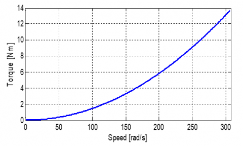
Torque – speed characteristic. Figure 3 indicates that the torque increases rapidly depending on the speed of rotation of the DSIM and it confirms the quadratic relation which exists between the torque of the pump and its rotation speed.
Since the starting torque is limited to the friction torque of the pump at zero speed, the pump requires a minimum speed at a given Hmt, to obtain a non-zero starting flow [24].
The theoretical characteristic of a centrifugal pump is a parabola starting from the origin and proportional to the square of the speed.
Figure 3. Characteristic torque – speed
Flow – speed characteristic. The pump must be driven at a certain speed for it to provide flow.
Indeed, before reaching this level of speed, that is to say a value of 150 rad/s, the piping of the pump does not provide any flow, then, the flow increases with the increase in the speed of rotation. Figure 4 shows the variation of the flow as a function of the speed and it should be noted that they are directly proportional.
The amount of energy corresponds to the speed and the faster the wheel turns or the larger the wheel, the higher the speed of the liquid at the tip of the blade and the greater the energy transmitted to the liquid.
Figure 4. Characteristic flow – speed
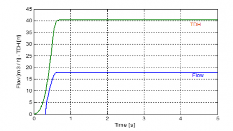
Flow and TDH characteristic. For water, TDH is simply the pressure head difference between the inlet and outlet of the pump, if measured at the same elevation and with inlet and outlet of equal diameter.
Figure 5. Characteristic flow – TDH
TDH is the total equivalent height that a fluid is to be pumped, taking into account friction losses in the pipe.
Figure 5 reveals that the variation of TDH is similar to that of the speed and the pump provides a flow only after a delay, equivalent to the time it takes for the pump to reach a certain speed of 151 rad/s.
4.1.2 DSIM characteristics
T6 is the transformation matrix calculated on the basis of the six healthy phases of DSIM which are only two three-phase systems offset by π / 6 between them.
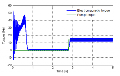
Figure 6 reveals that at start-up, the torque takes on a vibratory form and reaches values close to 80 Nm, then after 0.3 s at 40 Nm, the vibrations fade before reaching a no-load value of Tr = 0.32 Nm. This torque value corresponds to the without load losses and the mechanical friction losses.
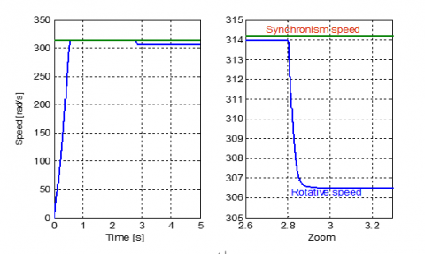
Figure 7 shows the evolution of the speed of rotation of the DSIM which, at the start, increases in a quasi linear way to reach the speed of 313.83 rad/s very close to the synchronism speed which is 314.16 rad/s.
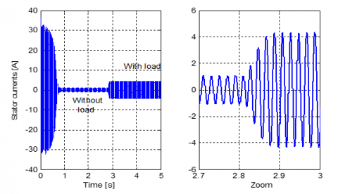
At starting, the DSIM absorb current of five times the nominal current, i.e. 30A and in the case of excessive repetitions, these start-up currents can be at the origin of the destruction by heating of the windings of the stator of the DSIM. Figure 8 indicates that the steady state is reached after a period of 0.6 s and the DSIM absorbs a current of 0.88 A without load; when connecting the load, the motor absorbs more current from the network which oscillates around 3.5 A.
Figure 6. Electromagnetic & pump torques (no defect)
Figure 7. Rotative & synchronism speed (no defect)
Figure 8. Stator electric current (normal mode)
4.2 Defect of phase
When a fault occurs on one phase, the transformation matrix is calculated on the basis of the five healthy phases and is given by:
$\left[T_{5}\right]=\left[\begin{array}{lllll}+0.6124 & -0.3536 & -0.6124 & -0.3536 & -0.0000 \\ +0.2887 & +0.5000 & +0.2887 & -0.5000 & -0.5774 \\ +0.4487 & -0.4967 & +0.7281 & +0.0129 & +0.1471 \\ +0.5330 & +0.3198 & -0.0911 & +0.7611 & -0.1613 \\ +0.2372 & +0.5253 & +0.0570 & -0.2133 & +0.7868\end{array}\right]$
The DSIM continues to rotate while providing torque to its shaft which will be reduced compared to its nominal value.
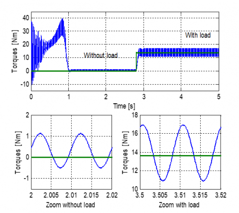
Figure 9. Electromagnetic & Pump torques (one phase)
Figure 10. Stator electric current (one phase)
With this faulty phase, at startup, the torque of the machine decreases considerably compared to its value where all the feeding phases are healthy.
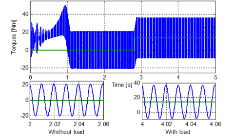
The torque reaches a peak of 47.2 Nm, and then the vibrations fade after 0.75 s before reaching a float value between 0.6 Nm and 1.2 Nm corresponding to the no-load losses and the mechanical losses by friction.
Figure 9 shows that when the load is connected, the torque goes to the disturbed and wavy float value between 11.8 Nm and 16.8 Nm around the value of the resisting torque. The frequency of the oscillations is twice that of the supply currents.
The speed reaches the synchronism speed after 0.75 s, slower than that of a healthy operation and with a load this speed switches around 306 rad/s.
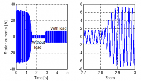
The zoom of Figure 10 shows that without load, the current increases to 1.1 A and during the coupling of the load the DSIM absorbs currents of 4.44 A.
4.3 Case of two faulty phases
The two faulty phases can be in the same star or in a different star.
4.3.1 Failure of two phases of the same star
The Sa2 and Sb2 phases are chosen to simulate a fault that could occur on two phases of the same star.
The transformation matrix is calculated based on the four healthy phases of the same star and is given by:
$\left[T_{4}\right]=\left[\begin{array}{llll}+0.8165 & -0.4082 & -0.4082 & -0.0000 \\ +0.0000 & +0.5477 & -0.5477 & -0.6325 \\ +0.5527 & +0.4235 & +0.6819 & -0.2238 \\ +0.1668 & +0.5950 & -0.2613 & +0.7416\end{array}\right]$
Figure 11 highlights the undulations of the torque no and with load. The torque stabilizes after 1 s, oscillating around 0.8 Nm without load and around 13.9 Nm with load. The value of the resistive torque is 13.6 Nm.
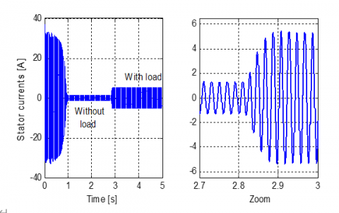
Figure 12 shows that at the start, strong currents are called reaching 35 A, then after the established regime, the DSIM absorbs 1.37 A without load. On the other hand, under load, the absorbed current increases and is around 5.8 A.
Note that small ripples are observed around the average speed of 305.60 rad/s and the rise time has increased to 1 s.
Figure 11. Torques evolution (two phases same star)
Figure 12. Stator electric current (two phases same star)
4.3.2 Two different star phases defect
Sa1 and Sc2 phases are chosen to simulate a fault that could occur on two phases of the different star.
The transformation matrix is calculated based on the four healthy phases of the same star and is given by:
$\left[T_{4}\right]=\left[\begin{array}{llll}+0.6124 & -0.3536 & -0.6124 & -0.3536 \\ +0.3536 & +0.6124 & +0.3536 & -0.6124 \\ +0.4082 & -0.5774 & +0.7041 & +0.0649 \\ +0.5774 & +0.4082 & -0.0649 & +0.7041\end{array}\right]$
Figure 13. Torques evolution (two phases different star)
After a start-up, Figure 13 shows that the torque reaches after 1 s, the value corresponding to the without load losses, and then the torque follows the setpoints, note that for speed, the rise time is 0.96 s and the speed is 305.95 rad/s.
With regard to the stator currents, Figure 14 relates that the results of this simulation are identical to those found for the case of two phases of the same star.
$\left[T_{3}\right]=\left[\begin{array}{lll}+0.7071 & +0.6124 & -0.3536 \\ +0.0000 & +0.5000 & +0.8660 \\ +0.7071 & -0.6124 & +0.3536\end{array}\right]$
Figure 14. Stator electric current (two phases different star)
4.3.3 Summary of the various defects of two phases
For operation with two faulty phases, Table 4 summarizes the possible combinations and describes the state of the torque.
Figure 15 shows the very wavy state of the torque in case when two phases defect. The harmfulness of the torque state on the performance of the DSIM is the reason why the control strategies described previously in section 2.5 are used for keep the torque constant, ridding it of ripples.
Figure 15. Torques evolution with very wavy torque
4.4 Case of three faulty phases
4.4.1 Defect of three phase of different star
The transformation matrix is calculated based on the three healthy phases and is given by:
$\left[T_{3}\right]=\left[\begin{array}{lll}+0.7071 & +0.6124 & -0.3536 \\ +0.0000 & +0.5000 & +0.8660 \\ +0.7071 & -0.6124 & +0.3536\end{array}\right]$
Figure 16 reveals that in this case, the speed-up time further increases to 1.5 s, then after application of the load, the DSIM decelerates and the speed oscillates around the value of 304.8 rad/s.
Figure 16. Speeds evolution (three phases different star)
Table 4. State of the torque with two defective phases
|
State of the torque |
Defective phases in same star |
Defective phases in different star |
|
Not wavy |
- |
(Sb2-Sc1), (Sa2-Sb1), (Sa1-Sc2) |
|
Wavy |
(Sb1-Sc1), (Sb2-Sc2), (Sa2- Sb2) |
(Sb1, Sc2) |
|
Very wavy |
(Sa1-Sc1), (Sa1-Sb1), (Sa2-Sc2) |
(Sc1- Sc2), (Sa2-Sc1), (Sb1- Sb2), (Sa1- Sb2), (Sa1-Sa2) |
The stator currents at startup reach 34 A before fading to a value of 1.7 A. Figure 17 shows then after application of the load, the demand increases to 7.65 A.
The fact that the phases do not belong to the same star, torque oscillations are observed when empty and under load as shown in the Figure 18.
Figure 17. Stator electric current (three phases different star)
Figure 18. Torques evolution (three phases different star)
4.4.2 Loss of a star
If a star is lost, it is only a three-phase system. The transformation matrix is calculated based on the loss of a star and is given by:
$\left[T_{3}\right]=\left[\begin{array}{lll}+0.8165 & -0.4082 & -0.4082 \\ +0.0000 & +0.7071 & -0.7071 \\ +0.5774 & +0.5774 & +0.5774\end{array}\right]$
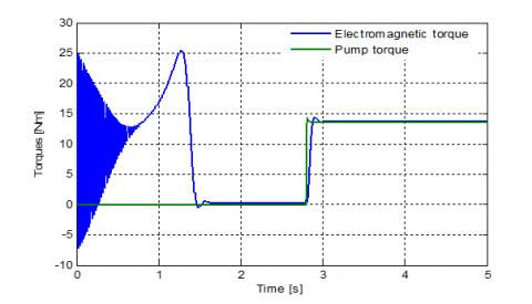
Figure 19 shows the vibratory form of the oscillating torque, before stabilizing at 0.31 Nm, value corresponding to the no-load losses. With the load, the torque follows the evolution of the resistant torque.
Figure 20 is a zoom which defines the evolution of the resistive torque and the electromagnetic torque and clearly shows that the couple follows its reference.
Figure 21 highlights the rise time which increases to 1.54s. On load, the DSIM decelerates to 304.8 rad/s.
The same behavior in healthy mode is observed with values divided by two.
Figure 18 and Figure 22 show that the current in the event of the loss of a star is identical to that of the loss of three different star phases.
Figure 19. Torques evolution (loss of a star)
Figure 20. Zoom in the evolution of torques (loss of a star)
Figure 21. Speeds evolution (loss of a star)
Figure 22. Stator electric current (loss of a star)
Table 5. Synthesis of the various simulations
|
|
Electromagnetic torque |
Rotation speed |
Current [A] |
|||
|
Defect phase |
Max [Nm] |
Stability time [s] |
Final [rad/s] |
Rise time[s] [s] |
No load |
With load |
|
Flawless |
49.35 |
0.65 |
306.3 |
0.62 |
0.88 |
3.55 |
|
5 phases |
47.20 |
0.75 |
306.1 |
0.76 |
1.10 |
4.50 |
|
2 phases same star |
39.80 |
1.00 |
305.6 |
1.00 |
1.37 |
5.80 |
|
2 various star phases |
33.73 |
1.00 |
605.6 |
1.00 |
1.32 |
5.51 |
|
Loss of a starstar |
25.40 |
1.50 |
304.8 |
1.50 |
1.73 |
7.65 |
|
3 various star phases |
25.50 |
1.50 |
304.8 |
1.56 |
1.80 |
7.95 |
4.5 Synthesis of the various simulations
4.5.1 Stator current
Without load, the absorbed current is 0.9 A with the six healthy phases and increases with the number of defective phases up to a value of 1.79 A with half-motor operation. When charging, the current is 3.55 A during normal operation and almost twice when a star is lost. This is because the DSIM absorbs the same current through its remaining three phases, i.e., the power is no longer segmented.
4.5.2 Rotation speed
Without load, the speed is reached after a period which increases with the increase of the number of defective phases. With load, the speed is 306.3 rad/s and decreases as the number of phases is reduced.
Figure 23 shows the decrease in speed. A difference of two rad/s is observed between normal mode and half-engine operation.
Figure 23. Comparison of speeds
4.5.3 Electromagnetic torque
In normal operation, the torque has a peak of around 49.35 Nm before stabilizing at its value corresponding to the no-load losses in a time of 0.65 s.
The loss of the phases leads to a decrease in the maximum value of the couple and an increase in the relaxation time.
Note that for operation with a single star, the value of the maximal torque is simply halved.
For operation with one or two stars, the torque has no ripple. In the event of a fault, undulations appear and increase with the number of defective arms of the inverter.
The Table 5 gives a comparison of the characteristic quantities of the DSIM during the various defects studied that may occur on the stator power phases.
During this small test, we could see that the DSIM can still rotate even in the case of loss of supply phases or short-circuit of the stator windings.
In degraded conditions, the couple finds themselves wavy or strongly wavy, which is very harmful to the drive system. Proposed techniques are adopted to deal with this kind of inconvenience. On the other hand the absorbed current increases and can reach double its nominal value, reason for which, it is necessary well to dimension the coils of the DSIM.
Depending on the field of use, it is possible to guarantee satisfactory operation by using powerful computers which, in real time, provide the appropriate control.
This operation must ensure a torque without ripples and a speed necessary for the load, while controlling the current demand which must satisfy an operation, without overheating, of the motor and avoid short-circuits of the turns of the stator windings.
After this analysis, it turns out that the DSIM, thanks to its flexibility, is widely used in military applications and in embedded applications, and may replace three-phase motors in the near future
In perspective, it is possible to study this engine in degraded mode without having to use a neutral connection.
|
COVID 19 |
Corona virus December 2019 |
|
|
DC/AC |
Inverter |
|
|
DC/DC |
Converter |
|
|
DSIM |
Dual stator induction motor |
|
|
IGBT |
Insulated-gate bipolar transistor |
|
|
MSAP-DE |
permanent magnet synchronous motor dual star |
|
|
d |
Axis direct index |
|
|
fr |
Coefficient of friction |
|
|
iai, ibi, ici |
Currents of star i |
|
|
irα, irβ |
Rotor current (α & β axis) |
|
|
Isα, isβ |
Stator current (α & β axis) |
|
|
iz1, iz2, iz3 |
Fictitious currents in space Z |
|
|
J |
Moment of inertia |
|
|
Kr |
Proportionality coefficient |
|
|
K0, K1, K2 |
pump constants |
|
|
Lr |
Rotor inductor |
|
|
Lsd, Lsq |
Direct and quadratic stator inductors |
|
|
Md, Mq |
Direct and quadratic mutuals |
|
|
p |
Number of pole pairs |
|
|
Pmec |
Mechanical power |
|
|
q |
Axis quadratic index |
|
|
Q |
Flow |
|
|
Rr |
Rotor resistant |
|
|
Rs |
Stator resistant |
|
|
Tc |
Transformation matrix |
|
|
TDH |
Total dynamic head |
|
|
Tem |
Electromagnetic torque |
|
|
Tr |
Resistant torque |
|
|
Ts |
Static torque |
|
|
VZi |
Fictitious voltages in space Z |
|
|
Vα, Vβ |
Stator voltage (α & β axis) |
|
|
wr |
Rotation speed |
|
|
Greek symbols |
||
|
$\phi_{s \alpha}, \phi_{s \beta}$ |
Stator fluxes (α & β axis) |
|
|
$\phi_{r \alpha}, \phi_{r \beta}$ |
Rotor fluxes (α & β axis) |
|
|
Ω |
Angular speed of rotation |
|
[1] Ibrahim, A. (2009). Contribution au diagnostic de machines électro-mécaniques: Exploitation des signaux électriques et de la vitesse instantanée. Thèse de Doctorat, école doctorale Sciences, Ingénierie, Santé Diplôme délivré par l’Université Jean Monnet.
[2] Cao, W., Mecrow, B.C., Atkinson, G.J., Benett, J.W., Atkinson, D.J. (2012). Overview of electric motor technologies used for more electric aircraft (MEA). IEEE Transactions on Industrial Electronics, 59(9): 3523-3531. https://doi.org/10.1109/TIE.2011.2165453
[3] Shamsi-Nejad, M.A. (2007). Architectures d'alimentation et de commande d'actionneurs tolérants aux défauts. Régulateur de courant non linéaire à large bande passante. Thèse de Doctorat, Institut National Polytechnique de Lorraine.
[4] Bellara, A., Chabour, F., Barakat, G., Amara, Y., Maalioune, H., Nourisson, A., Corbin, J. (2016). Etude du fonctionnement dégradé d'une machine synchrone à aimants permanents double étoile pour un inverseur de poussée. Symposium de genie electrique: EF-EPF-MGE 2016, Grenoble, France.
[5] Moraes, T.J.D.S., Nguyen, N.K., Meinguet, F., Guerin, M., Semail, E. (2016). Commande en mode dégradé d’un entrainement comportant deux machines 6 phases en série. Symposium de génie électrique: EF-EPF-MGE 2016, Grenoble, France.
[6] Crevits, Y. (2009). Characterization and control of polyphase training in degraded mode. Doctorat de génie électrique, rapport de première année, école polytechnique Lille France.
[7] Williamson, S., Smith, S., Hodge, C. (2014). Fault tolerance in multiphase propulsion motors. Journal of Marine Engineering and Technology, 3(1): 3-7. https://doi.org/10.1080/20464177.2004.11020174
[8] Kestelyn, X. (2003). Modélisation vectorielle multi machines pour la commande des ensembles convertisseurs-machines polyphasées. Thèse de doctorat en génie électrique à l’université de Lille 1.
[9] Bonnett, A.H., Soukup, G.C. (1992). Cause and analysis of stator and rotor failures in three-phase squirrel-cage induction motors. IEEE Transactions on Industry Applications, 28(4): 921-937. https://doi.org/10.1109/28.148460
[10] Bigret, R., Féron, J.L. (1995). Diagnostic, Maintenance Et Disponibilité Des Machines Tournantes. Edition Masson.
[11] Bonnett, A.H. (2000). Cause ac motor failure analysis with a focus on shaft failures. IEEE Transactions on Industry Applications, 36(5): 1435-1448. https://doi.org/10.1109/28.871294
[12] Huangsheng, X., Toliyat, H.A, Peteren, L.J. (2002). Five-phase induction motor drives with DSP based control system. IEEE Transactions on Power Electronics, 17(4): 524-533. https://doi.org/10.1109/TPEL.2002.800983
[13] Kianinezhad, R., Nahid-Mobarakeh, B., Baghli, L., Betin, F., Capolino, G.A. (2008). Modeling and control of six-phase symmetrical induction machine under fault condition due to open phases. IEEE Transactions on Industrial Electronics, 55(5): 1966-1977. https://doi.org/10.1109/TIE.2008.918479
[14] Zhao, Y., Lipo, T.A. (1996). Modeling and control of a multi-phase induction machine with structural unbalance. IEEE Transactions on Energy Conversion, 11(3): 570-577. https://doi.org/10.1109/60.537009
[15] Khaldi, L., Iffouzar, K., Ghedamsi, K., Aouzellag, D. (2019). Performance analysis of five-phase induction machine under unbalanced parameters. Journal Européen des Systèmes Automatisés, 52(5): 521-526. https://doi.org/10.18280/jesa.520512
[16] Welchko, B.A., Jahns, T.M. (2002). IPM Synchronous machine drive response to a single phase open circuit fault. IEEE Transaction on Power Electronics, 17(5): 764-771. https://doi.org/10.1109/TPEL.2002.802180
[17] Figueroa, J., Cros, J., Viarouge, P. (2003). Poly-phase PM brushless DC motor for high reliability application. September, Toulouse, CDROM, EPE.
[18] Robert-Dehault, E., Benkhoris, M.F., Semail, E. (2002). Study of 5-phases synchronous machine fed by PWM inverters under fault conditions. CDROM, ICEM.
[19] Hirtz, J.M. (1991). Les stations de pompage d’eau. 6e édition, Association Scientifique et Technique pour l’eau et l’environnement, éditions Lavoisier.
[20] Xu, H., Toliyat, H.A., Peteren, L.J. (2001). Modeling and control of five-phase induction motor under asymmetrical fault conditions. Electric Machines & Power Electronics Laboratory Texas A&M University.
[21] Mukund, R.P. (1999). Wind and Solar Power Systems. PhD, université Merchant Marine.
[22] Benkhoris, M.F., Tali-Maamar, N., Terrien, F. (2002). Decoupled control of double star synchronous motor supplied by PWM inverter: simulation and experimental results. Laboratoire Atlantique de recherche au génie Electrique (LARGE-GE44)-France.
[23] Royer, J., Djiako, T. (1998). Le Pompage Photovoltaïque. Manuel de cours à l’intention des ingénieurs et des techniciens, université d’Ottawa /EIER /CREPA.
[24] Martin, J.P., Meibody-Tabar, F., Davat, B. (2000). Multiple phase permanent magnet synchronous machine supplied by VSIS, working under fault conditions. CDROM, IAS.