Weiliang Zhang
© 2020 IIETA. This article is published by IIETA and is licensed under the CC BY 4.0 license (http://creativecommons.org/licenses/by/4.0/).
OPEN ACCESS
The purpose of this paper mainly explores the vibration resonance of the biological enzyme system with time delay, velocity feedback, and displacement feedback, under the excitation of signals with different frequencies and periods. Under approximate conditions, the fast and slow variables were separated to obtain the analytical solution of the system. the approach were theoretical analysis and numerical analysis show that the response amplitude gain of the biological enzyme system to low-frequency signal has two periodical relationships with the time delay: the period of low-frequency signal and that of high-frequency signal. The numerical results indicated that, the response amplitude gain is greatly affected by the symmetry and scale of the amplitudes, displacement response strengths, velocity response strengths of low- and high-frequency signals. For example, when the nonlinear term of the system μ=0.001, the response amplitude gain Q first increases, then decrease, and finally rebounds, with the growth of the frequency f of low-frequency signal; when μ=0, Q increases significantly with the growth of f, and the increasing rate grows proportionally; When the strength of displacement feedback u=0.08 and that of velocity feedback v=0.01 (that is, u and v are unequal), the change scope of amplitude gain Q widens. The research results shed important new light on vibration resonance of biological enzyme systems.
time delay, biological enzyme system, vibration resonance, amplitude gain
With the rapid development of modern engineering technology, nonlinear systems have attracted much attention in the academia, thanks to their application value in such fields as brain dynamics, laser physics, acoustics, communication, and system vibration [1-4].
As a typical nonlinear system, the van der Pol equation $\ddot{y}-\mu\left(1-y^{2}\right) \dot{y}+y=0$ was originally used to study the oscillation effect of transistors in the circuit. If added with cx6 and the excitation signal Fcos(wt), the equation will become a van der Pol oscillator with three limit cycles, and suffer from resonance, bifurcation and chaos [5-8].
If feedback term ux(t-τ) and time lag $v \dot{x}(t-\tau)$ are added, the van der Pol oscillator with three limit cycles can be used to simulate the response of enzymatic substrate in brain wave activity and the heart beat circuit [9-14].
Coupled with restoring force$2 K_{2}\left(1-\frac{L}{\sqrt{X^{2}+a^{2}}}\right)$, velocity feedback $\gamma_{v} \dot{X}(T-\delta)$, and displacement feedback $\gamma_{d} X(T-\delta)$ and damping, the van der Pol equation is capable of simulating the quasi-zero stiffness vibration problem in mechanical systems [15-20].
This paper introduces time-delay feedback and high- and low-frequency excitation signals to Q.Guo model, and explores how the vibration resonance of biological enzyme system varies with time delays, velocity feedback, and displacement feedback, under the excitation signals of different frequencies and periods. Next, the biological enzyme system was numerically analyzed by the Runge–Kutta method, aiming to disclose the effect of each parameter on the amplitude gain of the system response.
The biological enzyme system was simulated by a van der Pol equation with displacement feedback, velocity feedback, time delay, and high- and low-frequency excitation signals:
$\begin{align} & \ddot{x}=\mu \left( 1-{{x}^{2}}+\alpha {{x}^{4}} \right)\dot{x}-x \\ & +ux(t-\tau )+v\dot{x}(t-\tau )+{{F}_{w}} \\ \end{align}$ (1)
where, μ is a positive parameter that regulates the nonlinearity of the system; α is a positive parameter that measures the degree of ferroelectric instability of the system; u and v are the strength of the displacement feedback and the velocity feedback, respectively; x is proportional to the number of enzyme molecules in the excited polar state; $\dot{x}$ is the change rate of the number of excited enzyme molecules; $F_{w}=f \cos (w t)+F \cos (\Omega t)$ is the external excitation signal, with f being the amplitude of low-frequency excitation signal, w being the frequency of low-frequency excitation signal, F being the amplitude of high-frequency excitation signal, and Ω being the frequency of high-frequency excitation signal.
Without considering external excitation and feedbacks (u=v=0, and F=f=0), Eq. (1) can be rewritten as:
$ddot{x}=\mu \left( 1-{{x}^{2}}+\alpha {{x}^{4}} \right)\dot{x}-x$ (2)
Eq. (2) has a fixed point $(x, \dot{x})=(0,0)$, whose stability depends on eigenvalues $\operatorname{det}\left(\begin{array}{cc}\lambda & 1 \\ 1 & \lambda-\mu\end{array}\right)=\lambda^{2}-\mu \lambda-1$=0 and $\lambda=\frac{\mu \pm \sqrt{\mu^{2}+4}}{2}$. According to the Routh-Hurwitz stability criterion, when μ<0, the characteristic equation has a pair of conjugate complex roots with negative real parts. Therefore, the system converges μ<0 and diverges at μ>0.
When μ=-0.025 (Figure 1a), x gradually approaches and eventually stabilizes at the fixed point (0,0). When μ=0.025 (Figure 1c), x gradually deviates from the fixed point, indicating that the system is unstable.
Comparing Figures 1b and 1d, it can be seen that when the system is discrete and converged, the cluster degree of Figure 1b differs greatly from that of Figure 1d. In Figure 1b, after the phase point deviated from the limit cycle under disturbance, the new phase trajectory still gradually approaches the limit cycle; In Figure 1d, after the phase point deviated from the limit cycle under disturbance, the new phase trajectory gradually deviates from the limit cycle. Therefore, the limit cycle in Figure 1b corresponds to a stable system, while that in Figure 1d corresponds to an unstable system.
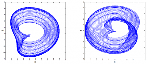
If added with feedbacks and excitation signals, the system will become more complex. Taking $y=\dot{x}$ and x in equation (1) as the vertical and horizontal axes, the feedbacks and excitation signals can be introduced simultaneously. The phase trajectory curves of the system at v=0.01 and v=0 can be displayed in Figures 2a and 2b, respectively. Obviously, the simultaneous addition of feedbacks and excitation signals has a great impact on the phase trajectory curves of the original system.
Figure 1. Time history and phase trajectory curves ( $u=0.01, v=0.01, y=\dot{x}$,)
Figure 2. Phase trajectory curves of system (1) $(\tau=0, \alpha=0.14, u=0.01)$
If μ is very small, only high-frequency signal was considered (f=0). Then, Eq. (1) can be simplified as:
$\ddot{x}=-x+u x(t-\tau)+v \dot{x}(t-\tau)+F \cos (\Omega t)$ (3)
According to T.Yang, $x(t-\tau)$ and $\dot{x}(t-\tau)$ in Eq. (3) can be approximated by Eqns. (4) and (5), resulting in Eq. (6):
$x(t-\tau) \approx \varepsilon \wedge_{1}(\Gamma) \cos [w(t-\tau)]-\varepsilon \wedge_{2}(\Gamma) \sin [w(t-\tau)]$
$=\varepsilon \wedge_{1}(\Gamma)[\cos (w t) \cos (w \tau)+\sin (w t) \sin (w \tau)]-\varepsilon \wedge_{2}(\Gamma)[\sin (w t) \cos (w \tau)-\cos (w t) \sin (w \tau)]$
$=\left[\varepsilon \wedge_{1}(\Gamma) \cos (w t)-\varepsilon \wedge_{2}(\Gamma) \sin (w t) \cos (w \tau)\right] \cos (w \tau)-\left[-\varepsilon \wedge_{1}(\Gamma) \sin (w t)-\varepsilon \wedge_{2}(\Gamma) \cos (w t)\right] \cos (w \tau)$
$=\left[\varepsilon \wedge_{1}(\Gamma) \cos (w t)-\varepsilon \wedge_{2}(\Gamma) \sin (w t)\right] \cos (w \tau)-\left[-\varepsilon w \wedge_{1}(\Gamma) \sin (w t)-\varepsilon \wedge_{2}(\Gamma) \cos (w t)\right] \frac{\sin (w t)}{w}$
$=x \cos (w \tau)-\frac{\dot{x} \sin (w \tau)}{w}$ (4)
$\dot{x}(t-\tau) \approx \varepsilon \wedge_{1}(\Gamma) \sin [w(t-\tau)]-\varepsilon \wedge_{2}(\Gamma) \cos [w(t-\tau)]$
$=\varepsilon \wedge_{1}(\Gamma)[\sin (w t) \cos (w \tau)-\cos (w t) \sin (w \tau)]-\varepsilon \wedge_{2}(\Gamma)[\cos (w t) \cos (w \tau)+\sin (w t) \sin (w \tau)]$
$=\left[\varepsilon \wedge_{1}(\Gamma) \cos (w t)-\varepsilon \wedge_{2}(\Gamma) \sin (w t)\right] w \sin (w \tau)+\left[-\varepsilon \wedge_{1}(\Gamma) \sin (w t)-\varepsilon \wedge_{2}(\Gamma) \cos (w t)\right] \cos (w \tau)$
$=\left[\varepsilon \wedge_{1}(\Gamma) \cos (w t)-\varepsilon \wedge_{2}(\Gamma) \sin (w t)\right] w \sin (w \tau)+\left[-\varepsilon w \wedge_{1}(\Gamma) \sin (w t)-\varepsilon \wedge_{2}(\Gamma) \cos (w t)\right] \cos (w \tau)$
$=x w \sin (w \tau)+\dot{x} \cos (w \tau)$ (5)
$\ddot{x}=-x+u\left[x \cos (\Omega \tau)-\frac{\dot{x} \sin (\Omega \tau)}{\Omega}\right]+v[x \Omega \sin (\Omega \tau)+\dot{x} \cos (\Omega \tau)]+F \cos (\Omega t)$ (6)
The analytical solution of Eq. (6) can be obtained or the numerical solution of that equation can be solved by the Runge–Kutta method, which produces the relationship between time delay τ and high-frequency time series. As shown in Figure 3, when the time delay τ=0, the amplitude of the time curve increases with the elapse of time, and the curve tends to diverge; when the time delay τ=0.5, the amplitude of the time curve increases slowly with the elapse of time, and the curve shows a periodic feature; when the time delay τ=1.2, the amplitude of the time curve attenuates with the elapse of time, and the curve tends to converge; when the time delay τ=2, the amplitude of the time curve attenuates with the elapse of time, and the curve tends to converge and shows a periodic feature.
Figure 3. Influence of time delay τ on high-frequency time series
According to Eq. (6), the system response is mainly caused by the high-frequency signal. Considering the influence of nonlinear terms, the solution of Eq. (6) can be defined as:
$x(t)=\sum_{i=1}^{\infty}\left[m_{i} \sin (i \Omega t)+n_{i} \cos (i \Omega t)\right]$
$=\sum_{i=1}^{\infty} C_{i} \sin \left(i \Omega t+\phi_{i}\right)$ (7)
where, $C_{i}=\sqrt{m_{i}^{2}+n_{i}^{2}}, \phi_{i}=\operatorname{arct} \tan \frac{n_{i}}{m_{i}}$. Assuming that i=1, the equations of m1 and n1 can be obtained by substituting the hypothetical solution of Eq. (7) into Eq. (6). Through analysis, it is easy to learn that the solutions of coefficients m1 and n1 are both functions about $f[\Omega, F, \sin (\Omega t), \cos (\Omega t)]$. Then, the coefficient C1 determined by m1 and n1 must be a function about $f[\Omega, F, \sin (\Omega t), \cos (\Omega t)]$.
Hence, $C_{1}=f[\Omega, F, \sin (\Omega t), \cos (\Omega t)]$ holds. Then, it is not difficult to prove that:
$C_{1}\left(\tau+\frac{2 \pi}{\Omega}\right)$
$=f\left[\Omega, \mathrm{F}, \sin \left(\Omega\left(\tau+\frac{2 \pi}{\Omega}\right)\right), \cos \left(\Omega\left(\tau+\frac{2 \pi}{\Omega}\right)\right)\right]$
$=f[\Omega, \mathrm{F}, \sin (\Omega \tau+2 \pi), \cos (\Omega \tau+2 \pi)]=C_{1}(\tau)$ (8)
In other words, the solution determined by Eq. (7) is a function about $\frac{2 \pi}{i \Omega}$, with the minimum positive period of $\frac{2 \pi}{\Omega}$.
To verify the above result, it is assumed that u=v=0.01, F=2, Ω=5, x1=x and $x_{2}=\dot{x}$, in Eq. (6). Then, we have $X=\left(\begin{array}{l}x_{1} \\ x_{2}\end{array}\right)=\left(\begin{array}{l}x \\ \dot{x}\end{array}\right)$. Reducing the second-order derivative to the first order, we have:
$\dot{X}=\left(\begin{array}{c}\dot{x}_{1} \\ \dot{x}_{2}\end{array}\right)=\left(\begin{array}{c}x_{2} \\ \mu\left(1-x_{1}^{2}+\alpha x_{1}^{4}\right) x_{2}+u x(t-\tau) \\ +v x_{2}(t-\tau)+F \cos (\Omega t)\end{array}\right)$
Under the initial condition of $X_{0}=\left(\begin{array}{c}x_{1}(0) \\ x_{2}(0)\end{array}\right)=\left(\begin{array}{c}0 \\ -1\end{array}\right)$, the above analysis result can be verified by solving the numerical solution of differential Eq. (6) with the fourth-order Runge-Kutta method (9):
$k_{1}=f(t(i), y(i), z(i))$
$L_{1}=g(t(i), y(i), z(i))$
$k_{2}=f\left(t(i)+h / 2, y(i)+h / 2 \times k_{1}, z(i)+h / 2 \times L_{1}\right)$
$L_{2}=g\left(t(i)+h / 2, y(i)+h / 2 \times k_{1}, z(i)+h / 2 \times L_{1}\right)$
$k_{3}=f\left(t(i)+h / 2, y(i)+h / 2 \times k_{2}, z(i)+h / 2 \times L_{2}\right)$
$L_{3}=g\left(t(i)+h / 2, y(i)+h / 2 \times k_{2}, z(i)+h / 2 \times L_{2}\right)$
$k_{4}=f\left(t(i)+h, y(i)+h \times k_{3}, z(i)+h \times L_{3}\right)$
$L_{4}=g\left(t(i)+h, y(i)+h \times k_{3}, z(i)+h \times L_{3}\right)$
$y(i+1)=y(i)+h / 6 \times\left(k_{1}+2 \times k_{2}+2 \times k_{3}+k_{4}\right)$
$z(i+1)=z(i)+h / 6 \times\left(L_{1}+2 \times L_{2}+2 \times L_{3}+k_{4}\right)$ (9)
Using the Fourier coefficient at the high-frequency signal to measure the degree of vibration resonance, the amplitude gain can be defined as:
$\mathrm{Q}(\Omega)=\sqrt{\mathrm{B}_{s}^{2}+\mathrm{B}_{\mathrm{c}}^{2}} / \Omega$ (10)
where, $B_{s}=\frac{2}{m T} \int_{0}^{m T} x(t) \sin (\Omega t) d t$; $B_{c}=\frac{2}{m T} \int_{0}^{m T} x(t) \cos (\Omega t) d t$; m is a positive integer.
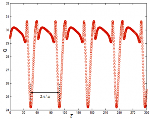
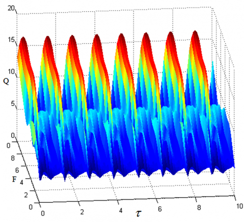
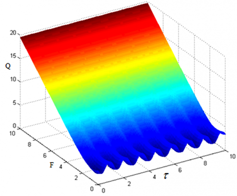
When System (1) contains both low- and high-frequency excitation signals, there is a periodic relationship between the response amplitude gain and the time delay. This analysis result can be verified by solving the numerical solution of system (1) with the fourth-order Runge-Kutta method (9). The numerical results (Figures 4 and 5) show that, for the high-frequency signal, when F and Ω are different, the minimum positive periods of the response amplitude gain and the time delay are both $\frac{2 \pi}{\omega}=\frac{2 \pi}{0.1}=62.8$; for the low-frequency signal, when f and ω are different, the minimum positive periods of the response amplitude gain and the time delay are both $\frac{2 \pi}{\Omega}=\frac{2 \pi}{5}=1.256$.
Figure 4. Periodic relationship between amplitude gain Q and time delay with high-frequency signal τ (ω=0.1, Ω=5, F=2, f=0.1)
Figure 5. Periodic relationship between amplitude gain Q and time delay with low-frequency signal (ω=0.1, Ω=5, F=2, f=0.1)
Figure 6. Analytical solution and numerical solution (F=2, u=0.01, v=0.01, Ω=2, f=0, τ=0)
Figure 6a presents the numerical solution obtained by the fourth-order Runge-Kutta method (9), while Figure 6b provides the analytical solution obtained by approximation. Figures 6a and 6b agree in the curve trend and periodic position. The only difference is that Figure 6a features the alternation between high and low amplitudes, while Figure 6b does not have this feature. The main reason is that the approximation method overlooks the nonlinear terms.
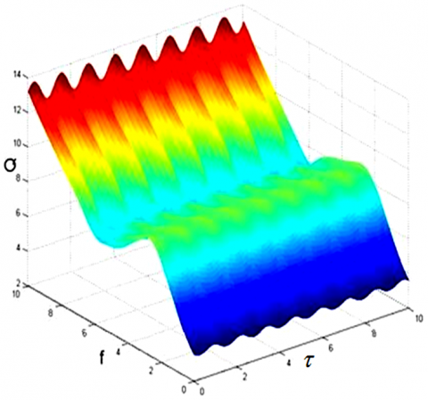
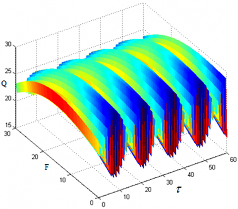
This section further explores the effects of each parameter in system (1) on the amplitude gain Q. Let F=2, u=v=0.01, Ω=5, and ω=0.1 in equation (1). The correlations of amplitude gain Q and the amplitude f and time delay τ of low-frequency signal can be obtained as Figure 7.
It can be seen that, along the axis of time delay τ, the periodic relationship between time delay τ and amplitude gain Q still exists. Along the axis of frequency f of low-frequency signal, when μ=0.001, Q first increases, then decrease, and finally rebounds, with the growth of f, along the axis of frequency f of low-frequency signal; when μ=0, the correlations of amplitude gain Q and the amplitude f and time delay τ of low-frequency signal can be obtained as Figure 8, Q increases significantly with the growth of f, and the increasing rate grows proportionally.
Figure 7. The correlations of amplitude gain Q and the amplitude f and time delay τ of low-frequency signal (μ=0.001, u=v=0.01)
Figure 8. The correlations of amplitude gain Q and the amplitude f and time delay τ of low-frequency signal (μ=0, u=v=0.01)
Figure 9. The correlations of amplitude gain Q and the amplitude F and time delay τ of high-frequency signal (μ=0.001, u=0.08, v=0.01)
Figure 10. The correlations of amplitude gain Q and the amplitude F and time delay τ of high-frequency signal (μ=0.5, u=v=0.01)
Figure 11. The correlations of amplitude gain Q and the amplitude F and time delay τ of high-frequency signal (μ=0.001, u=v=0.01)
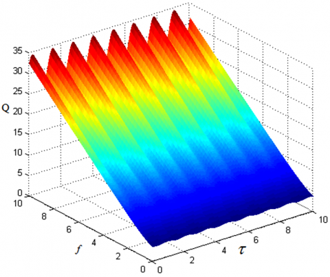
Let f=0.1, u=v=0.01, Ω=5, and ω=0.1 in equation (1). The correlations of amplitude gain Q and the amplitude F and time delay τ of high-frequency signal can be obtained as Figure 9.
It can be seen that, along the axis of time delay τ, the periodic relationship between time delay τ and amplitude gain Q still exists. The amplitude gain Q increases linearly with the growth of the frequency F of high-frequency signal. When the strength of displacement feedback u=0.08 and that of velocity feedback v=0.01 (that is, u and v are unequal), the change scope of amplitude gain Q widens, while the periodicity of the time delay’s τ direction is not affected.
Comparing Figures 10 and 11, it can be seen that, along the axis of time delay τ, the periodic relationship between time delay τ and amplitude gain Q still exists. When μ increases, the amplitude gain Q increases linearly with the growth in the frequency F of high-frequency signal; when μ=0.001, the change scope of Q is greater at μ=0.001 than at μ=0.5, provided that F values are the same.
Comparing Figures 12 and 13, it can be seen that, when the strength of displacement feedback u=0.01 and that of velocity feedback v=0.1 (that is, u and v are unequal), the change scope of amplitude gain Q widens, while the periodicity of the time delay’s τ direction is not affected.
Figure 12. The correlations of amplitude gain Q and the amplitude F and time delay τ of high-frequency signal (μ=0.1, u=v=0.01)
Figure 13. The correlations of amplitude gain Q and the amplitude F and time delay τ of high-frequency signal (μ=0.1, u=0.01, v=0.1)
This paper discusses the vibration resonance of the biological enzyme system with damping terms under the excitation of signals with different frequencies and periods. Through theoretical analysis and numerical analysis, the authors probed into the time series and response amplitude gain of the biological enzyme system, and examined the factors affecting the response amplitude gain. The numerical analysis was carried out by the fourth-order Runge-Kutta method. The results show that there are two different periods in the time series of the biological enzyme system: The period of low-frequency excitation signal, and that of high-frequency excitation signal. Further analysis shows that the response amplitude gain is greatly affected by the amplitudes, nonlinear parameters, and instabilities of high- and low-frequency signals:
When the strength of displacement feedback u=0.08 and that of velocity feedback v=0.01 (that is, u and v are unequal), the change scope of amplitude gain Q widens, while the periodicity of the time delay’s τ direction is not affected.
When μ increases, the amplitude gain Q increases linearly with the growth in the frequency F of high-frequency signal.
When μ=0.001, the change scope of Q is greater at μ=0.001 than at μ=0.5, provided that F values are the same.
When the strength of displacement feedback u=0.01 and that of velocity feedback v=0.1 (that is, u and v are unequal), the change scope of amplitude gain Q widens, while the periodicity of the time delay’s τ direction is not affected.
The project was supported by Natural Science Basic Research Plan in Shaanxi province of China (Program No. 2019JQ-896). Scientific research program funded by Shaanxi Provincial Education Department of China (Program No.19JK0034).
[1] Deng, B., Wang, J., Wei, X. (2009). Effect of chemical synapse on vibrational resonance in coupled neurons. Chaos: An Interdisciplinary Journal of Nonlinear Science, 19(1): 013117. https://doi.org/10.1063/1.3076396
[2] Deng, B., Wang, J., Wei, X., Yu, H., Li, H. (2014). Theoretical analysis of vibrational resonance in a neuron model near a bifurcation point. Physical Review E, 89(6): 062916. 10.1103/PhysRevE.89.062916
[3] Kaiser, F., Eichwald, C. (1991). Bifurcation structure of a driven, multi-limit-cycle van der Pol oscillator (i): The superharmonic resonance structure. International Journal of Bifurcation and Chaos, 1(2): 485-491. https://doi.org/10.1142/S0218127491000385
[4] Eichwald, C., Kaiser, F. (1991). Bifurcation structure of a driven multi-limit-cycle van der pol oscillator (ii): Symmetry-breaking crisis and intermittency. International Journal of Bifurcation and Chaos, 1(3): 711-715. https://doi.org/10.1142/S021812749100052X
[5] Hou, A., Guo, S. (2015). Stability and Hopf bifurcation in van der Pol oscillators with state-dependent delayed feedback. Nonlinear Dynamics, 79(4): 2407-2419. https://doi.org/10.1007/s11071-014-1821-3
[6] Fröhlich, H. (1968). Long‐range coherence and energy storage in biological systems. International Journal of Quantum Chemistry, 2(5): 641-649. https://doi.org/10.1002/qua.560020505
[7] Kaiser, F. (1978). Coherent oscillations in biological systems I. Zeitschrift für Naturforschung A, 33(3): 294-304. https://doi.org/10.1515/zna-1978-0307
[8] Kar, S., Ray, D.S. (2004). Large fluctuations and nonlinear dynamics of birhythmicity. EPL (Europhysics Letters), 67(1): 137. https://doi.org/10.1209/epl/i2003-10277-9
[9] Decroly, O., Goldbeter, A. (1982). Birhythmicity, chaos, and other patterns of temporal self-organization in a multiply regulated biochemical system. Proceedings of the National Academy of Sciences, 79(22): 6917-6921. https://doi.org/10.1073/pnas.79.22.6917
[10] Zhu, W.Q., Liu, Z.H. (2007). Response of quasi-integrable Hamiltonian systems with delayed feedback bang–bang control. Nonlinear Dynamics, 49(1-2): 31-47. https://doi.org/10.1007/s11071-006-9101-5
[11] Liu, Z.H., Zhu, W.Q. (2008). Asymptotic Lyapunov stability with probability one of quasi-integrable Hamiltonian systems with delayed feedback control. Automatica, 44(7): 1923-1928. https://doi.org/10.1016/j.automatica.2007.10.038
[12] Yang, T., Cao, Q. (2018). Delay-controlled primary and stochastic resonances of the SD oscillator with stiffness nonlinearities. Mechanical Systems and Signal Processing, 103: 216-235. https://doi.org/10.1016/j.ymssp.2017.10.002
[13] Jeevarathinam, C., Rajasekar, S., Sanjuan, M.A.F. (2011). Theory and numerics of vibrational resonance in Duffing oscillators with time-delayed feedback. Physical Review E, 83(6): 066205. https://doi.org/10.1103/PhysRevE.83.066205
[14] Fröhlich, H. (1968). Long-range coherence and energy storage in biological systems. International Journal of Quantum Chemistry, 2(5): 641-649. https://doi.org/10.1002/qua.560020505
[15] Decroly, O., Goldbeter, A. (1982). Birhythmicity, chaos, and other patterns of temporal self-organization in a multiply regulated biochemical system. Proceedings of the National Academy of Sciences, 79(22): 6917-6921. https://doi.org/10.1073/pnas.79.22.6917
[16] Ting, Y., Lin, H.P., Sung, Y.K., Yu, C.H. (2019). Design a composite piezoelectric motor using face-shear and longitudinal resonance vibration. Sensors and Actuators A: Physical, 290: 62-70. https://doi.org/10.1016/j.sna.2019.03.002
[17] Yang, S.W., Zhang, W., Hao, Y.X., Niu, Y. (2019). Nonlinear vibrations of FGM truncated conical shell under aerodynamics and in-plane force along meridian near internal resonances. Thin-Walled Structures, 142: 369-391. https://doi.org/10.1016/j.tws.2019.04.024
[18] Lu, S., Zheng, P., Liu, Y., Cao, Z., Yang, H., Wang, Q. (2019). Sound-aided vibration weak signal enhancement for bearing fault detection by using adaptive stochastic resonance. Journal of Sound and Vibration, 449: 18-29. https://doi.org/10.1016/j.jsv.2019.02.028
[19] Xiao, L., Zhang, X., Lu, S., Xia, T., Xi, L. (2019). A novel weak-fault detection technique for rolling element bearing based on vibrational resonance. Journal of Sound and Vibration, 438: 490-505. https://doi.org/10.1016/j.jsv.2018.09.039
[20] Usama, B.I., Morfu, S., Marquié, P. (2019). Numerical analyses of the vibrational resonance occurrence in a nonlinear dissipative system. Chaos, Solitons & Fractals, 127: 31-37. https://doi.org/10.1016/j.chaos.2019.06.028