Jiali Pi | Weiming Zhang | Shifu Zhang* | Chunming Pi | Changhua Xie
OPEN ACCESS
The motion control of robot manipulator is inseparable from the manipulator dynamics. However, the relevant literature often discusses dynamics model and control method separately. This paper attempts to design a good and feasible dynamics model to enhance the motion control of manipulator. Firstly, a dynamics model of the flexible manipulator was proposed through finite matrix analysis, based on the Lagrange’s dynamics equations under different control conditions. Based on the flexible dynamics model, two adaptive control systems were designed based on whether the interaction force is known. In the control stage, a separated controller was developed by applying the adaptive model and sliding mode principle. The stability and robustness of our control strategy were proved through Lyapunov’s method. Finally, several numerical tests were carried out the verify the feasibility and superiority of our control strategy. The research results provide new insights into the dynamic control of robots with varied load constraints and any degree of freedom (DOF).
flexible dynamics, Lagrange’s equation, adaptive control, manipulator
The robot, coupled by a mechanical system and a control system, exhibits a high nonlinearity [1]. During operation, the maximum acceleration of the robot is up to 3-5g, calling for a high precision in trajectory tracking [2]. For robot with a flexible structure, the excessive deformation of the manipulator, if not considered in the mathematical model, will have a great impact on the dynamic performance [3]. The flexible dynamics of the manipulator may cause errors in the interaction torque of the motor and the positioning of the end effector. For precision work, the positioning of the end effector should vibrate within a very small amplitude, ideally with no vibration at all [4]. To achieve precision control of robotic motions, the deformation of the flexible manipulator must be considered in the mathematical model and subjected to precise dynamics analysis [5, 6]. Traditionally, the dynamics of the connecting rod-type manipulator are described by partial differential equations in an infinite dimensional space, which is difficult to apply in system analysis and control design [7]. Therefore, this paper establishes the dynamics equation through the finite matrix analysis in the Lagrange’s equations.
In the dynamics equation, the manipulator is simultaneously constrained by the interaction force and the motion trajectory [8]. The two constraints exist in the cartesian space and the configuration space, respectively. Thus, it is not easy to design a force-displacement control for robot dynamics, which is not subjected to both constraints at the same time [9]. To solve the problem, various control methods have been developed, including position control, speed control, force and displacement hybrid control [10]. These methods can be roughly divided into classic control and modern control. The modern control approaches are extended from classic ones to further address the nonlinearity and uncertainty of the robot [11, 12].
In this paper, the Jacobian matrix is adopted to assign the force in cartesian space to the joint in configuration space. For the flexible manipulator, a dynamic control method was designed to ensure the stability of the interaction force control loop, whether in a known or unknown mode. The method can provide appropriate feedback for the precise control of the interaction force [13], and effectively guarantee the control quality without the measured interaction force.
This paper models the dynamics of a five degree-of-freedom (5DOF) flexible manipulator through finite matrix analysis. Firstly, the displacement of each joint of the manipulator was calculated through finite matrix analysis. Secondly, the dynamics model of the manipulator was established based on nodal displacement, according to the Euler–Bernoulli beam theory. Finally, the author obtained the Lagrange’s dynamics equation of the flexible manipulator.
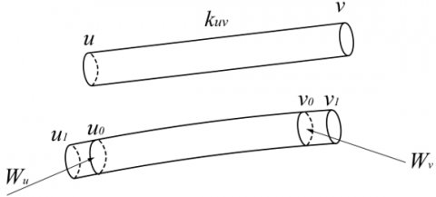
The flexible manipulator is equivalent to an inhomogeneous cylindrical member of constant cross-section, which satisfies the small deformation hypothesis of the Euler–Bernoulli beam theory. Figure 1 presents the deformation of the flexible manipulator and the joint equivalent model.
The center of the shoulder joint was taken as the origin of the fixed coordinate system $\mathrm{x}_{0} \mathrm{y}_{\mathrm{o}} \mathrm{z}_{\mathrm{o}} .$ In the moving coordinate system, the positions of the left end u before and after the manipulator deformation are denoted as $\mathrm{u}_{0}$ and $\mathrm{u}_{1}$, respectively. Let $\overrightarrow{\Delta p}$ be the projection of u in the fixed coordinate system, and $\overrightarrow{\mathrm{u}}=\left[\mathrm{x}_{\mathrm{u}}, \mathrm{y}_{\mathrm{u}}, \mathrm{z}_{\mathrm{u}}\right]^{\mathrm{T}}$ be the displacement vector of u, with $\mathrm{x}_{\mathrm{u}}$ be the $\mathrm{x}$ -axis coordinate of $\mathrm{u}$ in the fixed coordinate system. The symbols for the right end v are defined in the same manner (e.g. $\overrightarrow{\mathrm{v}}$ is the displacement vector of $\mathrm{v}$ ).
Figure 1. The deformation of the flexible manipulator and the joint equivalent model
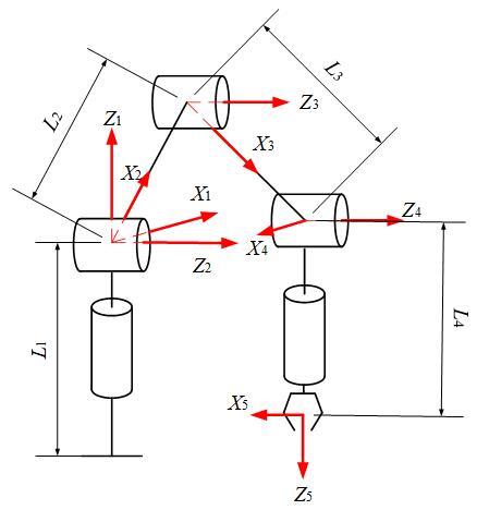
As shown in Figure $2,$ the manipulator mainly includes components like shoulder $\left(\mathrm{L}_{1}\right),$ elbow $\left(\mathrm{L}_{2}\right),$ arm $\left(\mathrm{L}_{3}\right),$ hand $\left(\mathrm{L}_{4}\right)$ and pedestal $\left(\mathrm{O}_{0}\right)[4]$
Figure 2. The mechanical model of the manipulator
Table 1. Parameters of the 5DOF manipulator
$\begin{array}{|c|ccccc|c|}\hline \text { Name } & {\text { Twist angle twist }_{i-1}} & {\text { Link length } a_{i-1}} & {\text { Link offset } d_{i}} & {\text { Joint angle } \theta_{i}} & {\text { Moment of inertia } I_{i}} \\ \hline 1 & {0} & {0} & {L_{1}} & {\theta_{1}} & {I_{1}} \\ {2} & {\frac{\pi}{2}} & {0} & {0} & {\theta_{2}} & {0} \\ {3} & {0} & {L_{2}} & {0} & {\theta_{3}} & {1_{2}} \\ {4} & {0} & {L_{3}} & {0} & {\theta_{4}} & {I_{3}} \\ 5 & {-\frac{\pi}{2}} &{0} & {L_{4}} & {\theta_{5}} & {I_{4}} \\ \hline\end{array}$
The parameters of the 5DOF flexible manipulator are listed in Table 1, where twisti-1 is the coordinate array on the twist angle of the hinge point.
The mapping $_{0}^{5} \mathrm{T}$ from the cartesian space to the configuration space can be expressed as a Denavit-Hartenber (D-H) matrix:
$_{0}^{5} \mathrm{T}=\left[\begin{array}{ll}{\mathrm{R}} & {\mathrm{P}} \\ {0} & {1}\end{array}\right]$ $=\left[\begin{array}{cccc}{r_{11}} & {r_{12}} & {r_{13}} & {x} \\ {r_{21}} & {r_{22}} & {r_{23}} & {y} \\ {r_{31}} & {r_{32}} & {r_{33}} & {z} \\ {0} & {0} & {0} & {1}\end{array}\right]$ (1)
$\left\{\begin{aligned} \alpha=\operatorname{atan} =2\left(\mathrm{r}_{32}, \mathrm{r}_{33}\right) \\ \beta=\operatorname{atan} 2\left(-\mathrm{r}_{31}, \sqrt{\mathrm{r}_{32}^{2}+\mathrm{r}_{33}^{2}}\right) \\ \gamma =\operatorname{atan} 2\left(\mathrm{r}_{21}, \mathrm{r}_{11}\right) \end{aligned}\right.$ (2)
$\left[\begin{array}{l}{\theta_{1}} \\ {\theta_{2}} \\ {\theta_{3}} \\ {\theta_{4}} \\ {\theta_{5}}\end{array}\right] \begin{array}{c}{^{_{0}^{5} \mathrm{T}}} \\{\rightarrow}\end{array} \left[\begin{array}{l}{x} \\ {y} \\ {z} \\ {\alpha} \\ {\beta} \\ {\gamma}\end{array}\right]$ (3)
Formula (2) describes the relationship between Euler angle and parameters in the D-H matrix.
2.1 Nodal displacement equation based on finite matrix analysis
The dynamics of the manipulator were analyzed through finite matrix analysis. The dynamic motions of the robot were transformed into the instantaneous static structure for mechanical analysis. In this way, the nodal displacement of the robot in each state was acquired, laying the basis for setting up the flexible dynamic equation.
Unlike the rigid mechanical strategy, the finite matrix analysis considers the elastic deformation, and converts the simple rigid multi-body dynamics model into an elastic model. In the new model, the manipulator at each moment can be viewed as a static structure with instantaneous motions. The stiffness of the manipulator can be described by an elastomeric equation that defines the linear relationship between the external force applied by a wrench w and the corresponding deflection ∆t. The elastomeric equation at an end can be expressed as:
$\mathrm{W}=\mathrm{K} \cdot \Delta \mathrm{t}$ (4)
where, $\mathrm{K}$ is a $6 \times 6$ stiffness matrix; $\Delta \mathrm{t}$ is a 6 -dimensional deflection vector (including translation $\Delta \mathrm{p}=[\Delta \mathrm{x}, \Delta \mathrm{y}, \Delta \mathrm{z}]$ and rotation $\Delta \varphi=[\Delta \alpha, \Delta \beta, \Delta \gamma] \text { components }) .$ Similarly, the external force $W$ is also a 6 -dimensional component (containing forces $\mathrm{F}=\left[\mathrm{F}_{\mathrm{x}}, \mathrm{F}_{\mathrm{y}}, \mathrm{F}_{\mathrm{z}}\right]$ and moments $\mathrm{M}=$ $\left.\left[\mathrm{M}_{\mathrm{x}}, \mathrm{M}_{\mathrm{y}}, \mathrm{M}_{\mathrm{z}}\right]\right)$
The elastomeric equation W can converts the inertial force and the external force on the truss into an equivalent nodal force on each node. This process is called the equivalent nodal force transform.
Substituting the equivalent nodal force and the stiffness matrix into formula (4), the nodal displacement ∆t can be derived from the nodal displacement and the constitutive relation of the material. The axial force and shear force of each member can be respectively obtained as:
$\begin{array}{c}{\mathrm{W}_{1}} \,\,\,\, {\Delta \mathrm{t}_{1}} \\ {\mathrm{W}_{2}} \,\,\,\, {\Delta \mathrm{t}_{2}} \\{\mathrm{W}_{3}=\mathrm{K} \Delta \mathrm{t}_{3}}\\ {\mathrm{W}_{4} \quad \Delta \mathrm{t}_{4}}\\ {\mathrm{W}_{5} \quad \Delta \mathrm{t}_{5}} \end{array}$ (5)
s.t.
$\left\{\begin{aligned} \Omega^{\mathrm{r}} \cdot\left(\Delta \mathrm{t}_{\mathrm{i}}-\Delta \mathrm{t}_{\mathrm{j}}\right) &=0 \\ \mathrm{W}_{\mathrm{i}}+\mathrm{W}_{\mathrm{j}}=0 & \\ \mathrm{\Omega}^{\mathrm{e} \cdot} \mathrm{W}_{\mathrm{j}}=\mathrm{k}_{\mathrm{q}} \cdot \Omega^{\mathrm{e}} \cdot\left(\Delta \mathrm{t}_{\mathrm{i}}-\Delta \mathrm{t}_{\mathrm{j}}\right) \\ \Omega^{\mathrm{e}} \cdot\left(\Delta \mathrm{t}_{\mathrm{i}}-\Delta \mathrm{t}_{\mathrm{j}}\right)=\xi \end{aligned}\right.$ (6)
where, $\xi$ is the amount of joint spring deformation; $\Omega$ is the geometric matrix of the manipulator; e is the elastic joint; $\mathrm{r}$ is the non-elastic joint; $\mathrm{k}_{\mathrm{q}}$ is stiffness matrix.
2.2 Dynamic equation of flexible manipulator
During the movement, the manipulator witness changes in its spatial position and potential energy of elastic deformation [14]. The finite matrix analysis was performed on the four links of the manipulator to obtain the generalized coordinates of the potential energy. The lengths of the links are denoted as L1, L2, L3 and L4, respectively. It is assumed that the elastic joint axis points to the Z-direction. Then, the angle between the adjacent links equals the rotation angle of the elastic joint $\theta_{i}$. The manipulator was defined in the xy plane for the Euler-Bernoulli beam model with a constant cross-section of A. To describe the potential energy of each Euler-Bernoulli link, the deflection control equation was solved as a differential equation, in the light of the load distributed on the link.
(1) Link equation based on Euler-Bernoulli beam model
Figure 3. Mechanical model of a link
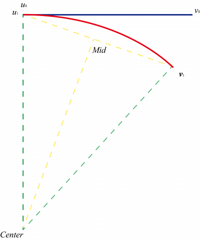
Figure 4. Deformation dynamics model of a link
Note: The blue line represents the original link, and the red line stands for the deformed link.
As shown in Figure 3, the Euler-Bernoulli beam theory assumes that the planar section remains through the deformation process. The displacement ∆v at the distance n of the intermediate axis of the link can be given by:
$\Delta \mathrm{v}=-\mathrm{n} \frac{\mathrm{d} \gamma_{\text {deflection }}}{\mathrm{d} \mathrm{l}}$ (7)
where, l and n are the coordinates in the axial direction and the normal direction, respectively. According to the deformation dynamics model in Figure $4, u_{1}$ is aligned to $u_{0},$ and the normal lines of $u_{1}$ and $v_{1}$ intersect each other at the center. Hence, the radius of curvature can be obtained. since the curvature of arc $\mathrm{u}_{0} \mathrm{v}_{1}$ is unknown, the midpoint Mid of the line segment $u_{0} v_{1}$ can be used as the normal to intersect the normal of $\mathrm{u}_{0} \mathrm{v}_{1},$ where $\mathrm{u}_{0} \mathrm{v}_{1}=\mathrm{v}_{0}+\overrightarrow{\Delta \mathrm{p}}$
$\left\{\begin{array}{c}{\overrightarrow{\mathrm{u}_{0} \mathrm{v}_{0}} \cdot \overrightarrow{\mathrm{u}_{0} \text { Center }}=0} \\ {\overrightarrow{\mathrm{u}_{0} \mathrm{v}_{1}} \cdot \overrightarrow{\mathrm{CenterM}_{1} \mathrm{d}}=0}\\ {\overrightarrow{Centeru_0} \cdot \overrightarrow{CenterM_1d}=\overrightarrow{CenterM_1d} \cdot \overrightarrow{Centerv_1}}\end{array}\right.$ (8)
It can be seen that $\mathrm{r}=\|$ Centeru $_{0} \|$, and the following can be obtained by approximating the differential equation of the deflection curve:
$\frac{\partial^{2} \gamma_{\text {deflection }}}{\partial 1^{2}}=\frac{1}{r}$ (9)
where, $\gamma_{deflection}$ is the deflection of the manipulator. The positive and shear strains of the link can be respectively defined as:
$\epsilon_{1}=\frac{\partial \mathrm{v}}{\partial \mathrm{l}}=-\mathrm{n} \frac{\partial^{2} \gamma_{\mathrm{deflection}}}{\partial \mathrm{l}^{2}}$; $\gamma_{\ln }=\frac{\partial \mathrm{v}}{\partial \mathrm{l}}+\frac{\partial \mathrm{v}}{\partial \mathrm{n}}=0$.
Then, the potential energy of elastic deformation of robotic links can be obtained as:
$\mathrm{E}_{\mathrm{p} 2}=\frac{1}{2} \int_{\mathrm{V}} \sigma_{1} \epsilon_{1} \mathrm{d} \mathrm{V}=\frac{1}{2} \int_{\mathrm{V}} \mathrm{E} \epsilon_{1}^{2} \mathrm{d} \mathrm{V}$ (10)
Substituting dV=dAdl into formula (10) and integrating in the l direction, we have:
$\mathrm{E}_{\mathrm{p} 2}=\frac{1}{2} \int_{0}^{\mathrm{a}} \mathrm{EI}_{\mathrm{i}}\left(\frac{\partial^{2} \gamma_{\text {deflection }}}{\partial \mathrm{l}^{2}}\right)^{2} \mathrm{d} \mathrm{l}$ (11)
where, $\mathrm{I}_{\mathrm{i}}=\int_{0}^{\mathrm{a}} \mathrm{n}^{2} \mathrm{d} \mathrm{Adl}$ is the moment of inertia of the cross-section $A$ of the $\operatorname{link} ; \mathrm{E}$ is the elastic modulus; $\mathrm{EI}_{\mathrm{i}}$ is the bending stiffness.
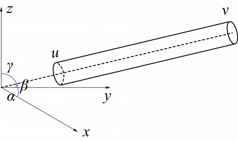
Figure 5. The dynamics model in the global coordinate system
As shown in Figure 5, the axial displacement depends on the axial vector:
$\overrightarrow{\mathrm{l}}=\Delta \mathrm{xi}+\Delta \mathrm{y} \mathrm{j}+\Delta \mathrm{zk}$ (12)
The norm of the axial vector can be described as:
$\|\overrightarrow{\mathrm{1}}\|=1=\sqrt{\Delta \mathrm{x}^{2}+\Delta \mathrm{y}^{2}+\Delta \mathrm{z}^{2}}$ (13)
where,
$\Delta \mathrm{x}=\operatorname{acos} \alpha, \Delta \mathrm{y}=\operatorname{acos} \beta, \Delta \mathrm{z}=\operatorname{acos} \gamma$
The differential equation of the link can be defined as:
$\mathrm{d} \mathrm{l}=\left(\frac{\partial \mathrm{l}}{\partial \alpha} \frac{\mathrm{d} \alpha}{\mathrm{d} \theta}+\frac{\partial \mathrm{l}}{\partial \beta} \frac{\mathrm{d} \beta}{\mathrm{d} \theta}+\frac{\partial \mathrm{l}}{\partial \gamma} \frac{\mathrm{d} \gamma}{\mathrm{d} \theta}\right) \mathrm{d} \theta \mathrm{d} \mathrm{v}$ (14)
Thus, formula (11) can be rewritten as:
$\mathrm{E}_{\mathrm{p} 2}=\frac{1}{2} \int_{0}^{\mathrm{a}} \mathrm{E} \mathrm{I}_{\mathrm{i}}\left(\frac{1}{\mathrm{r}}\right)^{2} \mathrm{d} \mathrm{l}$ (15)
Besides that of the link, the potential energy of elastic deformation of the joint was also taken into account. Considering the joint as a torsion spring, the dynamics model of the flexible joint can be established as:
$\mathrm{E}_{\mathrm{p} 3}=\frac{1}{2} \mathrm{I}_{\mathrm{m}}(\dot{\theta}-\Delta \varphi)^{2}+\frac{1}{2} \mathrm{k} \xi^{2}$ (16)
where, $\mathrm{I}_{\mathrm{m}}$ is the moment of inertia; $\theta$ is the actual rotation angle of the joint; $\xi$ is the deformation of the joint spring; $\mathrm{k}_{\mathrm{q}}$ is elastic stiffness coefficient of the flexible joint, which is equivalent to a nonlinear torsion spring. The energy equation of the elastic joint ensures the balance of all the components under rotation, and describes the laws of elasticity and inertia of the elastic joint.
(2) Lagrange’s energy dynamics equation
The kinetic energy of the flexible link can be described as:
$\mathrm{E}_{\mathrm{k}}=\frac{1}{2} \int_{0}^{\mathrm{a}} \rho(\mathrm{l}) \mathrm{i}^{\mathrm{T}} \mathrm{i} \mathrm{d} \mathrm{l}$ (17)
where, $\rho(1)$ is the axial density of the manipulator.
The total potential energy of the manipulator includes the potential energy of elastic deformation $\mathrm{E}_{\mathrm{p} 2}$ of the flexible joint, the torsion and the bending strain energy $\mathrm{E}_{\mathrm{p} 3}$ of the joint spring, and the gravitational potential energy $\mathrm{E}_{\mathrm{p} 1}:$
$\mathrm{E}_{\mathrm{p}}=\mathrm{E}_{\mathrm{p} 1}+\mathrm{E}_{\mathrm{p} 2}+\mathrm{E}_{\mathrm{p} 3}$ (18)
where, $\mathrm{E}_{\mathrm{p} 1}=\mathrm{mzg} ; \mathrm{z}=_{0}^{5} \mathrm{T}(\mathrm{z})$ is the mass concentration of the end. According to the structure of the manipulator, the generalized coordinate system is based on $\theta .$ Thus, the dynamics equation can be defined by the Lagrange equation:
$\mathrm{L}=\mathrm{E}_{\mathrm{k}}-\mathrm{E}_{\mathrm{p}}, \frac{\mathrm{d}}{\mathrm{dt}}\left(\frac{\partial \mathrm{L}}{\partial \dot{\theta}}\right)-\frac{\partial \mathrm{L}}{\partial \theta}=0$ (19)
The above formula combines the kinetic energy, potential energy, and gravitational potential energy of the manipulator to obtain the torque in the robotic configuration space. Hence, the dynamics equation can be rewritten as:
$\mathrm{M}(\theta) \ddot{\theta}+\mathrm{C}(\theta, \dot{\theta}) \dot{\theta}+\mathrm{G}(\theta)=\tau$ (20)
The dynamics equation considers a 5DOF manipulator operating in a rigid environment [14]. To control the dynamics adaptively, the control structure must be robust to the uncertainty in the model. Therefore, the model was further deduced as follows. When the manipulator is in contact with the environment, a contact force Fin is applied to the dynamics system [19]. Then, the dynamics equation of the manipulator in the configuration space can be expressed as:
$\mathrm{M}(\theta) \ddot{\theta}+\mathrm{C}(\theta, \dot{\theta}) \dot{\theta}+\mathrm{F}(\dot{\theta})+\mathrm{G}(\theta)=\tau+\mathrm{J}(\theta) \mathrm{F}_{\mathrm{in}}$ (21)
where, $\theta \in \mathrm{R}^{\mathrm{n}}$ is the generalized coordinate vector; $\mathrm{M}(\mathrm{q}) \in$ $\mathrm{R}^{\mathrm{n} \times \mathrm{n}}$ is the inertia matrix of the manipulator; $\mathrm{C}(\theta, \dot{\theta}) \in \mathrm{R}^{\mathrm{n}}$ is the centrifugal force and Coriolis forces/moments; $G(\theta) \in \mathrm{R}^{\mathrm{n}}$ is the gravity term; $\mathrm{F}(\dot{\theta}) \in \mathrm{R}^{\mathrm{n}}$ are the viscosity force and friction terms; $\tau \in R^{n}$ is the control torque; $J(\theta) \in R^{m \times n}$ is the Jacobian matrix; $\mathrm{F}_{\mathrm{in}} \in \mathrm{R}^{\mathrm{m}}$ is the interaction force in the cartesian space; n is the number of DOFs of the manipulator; m is the dimension in the cartesian space.
The manipulator control aims to adjust the robot motions based on the position and force constraints acquired by the observer. Therefore, the assembly operation can conform to the contact constraints and gradually correct the motion errors.
According to the above dynamics model, the control process faces severe time variation, coupling, nonlinearity and uncertainty. The influence of nonlinearity and uncertainty on control effect is particularly prominent under heavy load. To overcome the difficulties, the most suitable strategy is to implement control adaptively to the time-varying parameters [16].
3.1 Control plans
The general methods to derive the adaptive control algorithms mainly target rigid manipulators. This paper mainly pursues the stable control of flexible manipulator under force and displacement constraints. Therefore, the traditional dynamics equation must be reformulated before being applied to our research [17-19].
According to the mechanics control equation, the path of the manipulator described in formula (21) can be called the generalized trajectory, which consists of the motion, velocity and acceleration trajectories in configuration space. To prevent the acceleration feedback and the dilemma of compensation, the generalized trajectory tracking error was introduced to the control system:
$\mathrm{e}=\theta_{\mathrm{d}}-\theta$ (22)
where, $\theta_{\mathrm{d}}$ is the desired joint angle after nodal displacement.
The tracking error of the sliding surface can be described as:
$\mathrm{s}=\dot{\mathrm{e}}+\Lambda \mathrm{e}$ (23)
The derivative of the tracking error form the design matrix $\Lambda=\Lambda^{\mathrm{T}}>0, \Lambda \in \mathrm{R}^{\mathrm{n}}$. To reduce the dimension of the control object and avoid the acceleration feedback, formulas (22) and (23) can be combined into:
$\dot{\theta}=v-s$ (24)
where, $\mathrm{v}=\dot{\theta}_{\mathrm{d}}+\Lambda \mathrm{e}, \mathrm{v}$is an auxiliary signal. From the above formula, we have:
$\ddot{\theta}=\dot{\mathrm{v}}-\dot{\mathrm{s}}$ (25)
Substituting formulas (23) and (25) into formula (21), we have:
$\mathrm{M}(\theta) \dot{\mathrm{s}}=$$-\mathrm{C}(\theta, \dot{\theta}) \mathrm{s}+\mathrm{M}(\theta) \dot{\mathrm{v}}+\mathrm{C}(\theta, \dot{\theta}) \mathrm{v}+\mathrm{G}(\theta)-\mathrm{U}-\mathrm{J}(\theta) \mathrm{F}_{\mathrm{in}}$. (26)
For convenience, it is assumed that:
$\mathrm{M}(\theta) \dot{\mathrm{v}}+\mathrm{C}(\theta, \dot{\theta}) \mathrm{v}+\mathrm{G}(\theta)=\mathrm{f}$ (27)
where, $\mathrm{f} \in \mathrm{R}^{\mathrm{m}}$ is the nonlinear function of the control system. The value of $\hat{\mathrm{f}}(\theta)$ is determined by the adaptive identification agency. For control design, the linear expression of the manipulator can be written as:
$\mathrm{f}=\mathrm{Y}(\theta, \dot{\theta}, \mathrm{v}, \dot{\mathrm{v}}) \mathrm{p}$ (28)
where, $\mathrm{Y}(\theta, \dot{\theta}, \mathrm{v}, \dot{\mathrm{v}})$ is an adaptive regressor depending on the angular displacement and angular velocity of the manipulator; $\mathrm{p}$ is the vector of uncertain structural parameters. The form of $\mathrm{Y}(\theta, \dot{\theta}, \mathrm{v}, \dot{\mathrm{v}}) \mathrm{p}$ changes with the manipulator structure, so does the form of $\mathrm{p} .$ Being a function vector for motion parameters and deterministic structural parameters, $\mathrm{Y}(\theta, \dot{\theta}, \mathrm{V}, \dot{\mathrm{V}})$ has a deterministic value that can be calculated online. Obviously, once $\mathrm{Y}(\theta, \dot{\theta}, \mathrm{v}, \dot{\mathrm{v}})$ is written in linear form, then the problem is transformed into a computational problem. Then, the only task is to design an adaptive mechanism. The value of $\mathrm{Y}(\theta, \dot{\theta}, \mathrm{v}, \dot{\mathrm{v}})$ can be calculated after $\mathrm{p}$ is recognized.
Let $\hat{\mathrm{p}}$ be the valuation of $\mathrm{p} .$ Then, $\hat{\mathrm{f}}$ can be written as: $\hat{\mathrm{f}}=$ $\mathrm{Y}(\theta, \dot{\theta}, \mathrm{v}, \dot{\mathrm{v}}) \hat{\mathrm{p}}$.
Finally, the tracking error after wave filtering can be described as:
$\mathrm{M}(\theta) \dot{\mathrm{s}}=-\mathrm{C}(\theta, \dot{\theta}) \mathrm{s}+\mathrm{f}-\mathrm{U}-\mathrm{J}(\theta) \mathrm{F}_{\mathrm{in}}$ (29)
The function f depends on the model of the manipulator and the environment. The other influencing factors of this function include the inaccurate known parameters of the manipulator and the unknown stiffness of the environment. Hence, our control system should consider the traditional proportional-derivative (PD) control, i.e. $\hat{\mathrm{f}} \in \mathrm{R}^{\mathrm{m}}$ controls the nonlinearity of the compensated object, and the influence of the interaction force Fin.
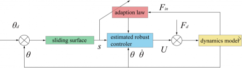
The adaptive position/force control for the flexible manipulator is illustrated in Figure 6 [20].
Figure 6. The adaptive position/force control
3.2 Separated control strategy
From the control plan, it can be seen that the interaction force is either unknown or known. If it is known, the interface force needs to be controlled precisely. Therefore, the control law must adapt to the type of the interaction force (Figure 7).
Figure 7. The proposed separated control strategy
Based on the dynamics model, the adaptive parameters were adopted to identify the control law. Taking the deviation from the desired interaction force as the main input, the control law of the known interaction force was designed based on the sliding mode structure, such that it is table under the Lyapunov’s method. Then, the parameters were estimated appropriately.
(1) The case of known interaction force
If the interaction force is known, the tracking error can be defined as:
$\mathrm{e}=\left[\theta_{\mathrm{d}}-\theta | \mathrm{F}_{\mathrm{d}}-\mathrm{F}_{\mathrm{in}}\right]$ (30)
The adaptive control law can be defined as:
$\mathrm{U}=\hat{\mathrm{f}}-\mathrm{J}(\theta) \mathrm{F}_{\mathrm{d}}+\mathrm{K}_{\mathrm{d}} \mathrm{s}$ (31)
Thus, the system description can be rewritten as:
$\mathrm{M}(\theta) \mathrm{\dot{s}}=-\mathrm{C}(\theta, \dot{\theta}) \mathrm{s}-\mathrm{K}_{\mathrm{d}} \mathrm{s}+\tilde{\mathrm{f}}+\mathrm{e}_{\text {force }}$ (32)
where, $\tilde{\mathrm{f}}=\mathrm{Y}(\theta, \dot{\theta}, \mathrm{v}, \dot{\mathrm{v}}) \tilde{\mathrm{p}}$ is the parameter estimation error; $\mathrm{F}_{\mathrm{d}}$ is the desired interaction force; e $_{\text {force is the deviation from the }}$ desired interaction force, $\mathrm{F}_{\mathrm{d}}-\mathrm{F}_{\mathrm{in}}$.
The above formula is a closed control loop for tacking error and parameter estimation error. To implement this adjustment law, p can be rewritten as:
$\hat{\mathbf{p}}=-\hat{\eta} \operatorname{sgn}\left(\sum_{\mathrm{j}=1}^{\mathrm{m}} \mathrm{s}_{\mathrm{j}} \mathrm{Y}_{\mathrm{j}}(\theta, \dot{\theta}, \mathrm{v}, \dot{\mathrm{v}})\right)$ (33)
$\dot{\hat{\eta}}=\Gamma \sum_{j=1}^{m} s_{j} Y_{j}(\theta, \dot{\theta}, v, \dot{v})$ (34)
where, $\mathrm{K}_{\mathrm{d}}$ is a positive definite array; $\Gamma>0$.
If the adaptive control law is applied to formulas (31) and (32), the tracking error will converge to zero.
(2) The case of unknown interaction force
If the interaction force is unknown, the interaction force was considered as an interference. Then, Fin was assumed to be related to and bounded by system state:
$\mathrm{F}_{\mathrm{in}} \leq \mathrm{d}_{0}+\mathrm{d}_{1} \mathrm{e}+\mathrm{d}_{2} \dot{\mathrm{e}}$ (35)
where, $\mathrm{d}_{0}>0 ; \mathrm{d}_{1}>0 ; \mathrm{d}_{2}>0$.
To avoid the impact of external perturbation on the control system, the switch rate of the sliding mode $\widehat{\sigma}_{0} \mathrm{S}+\widehat{\sigma}_{1} \operatorname{sgn}(\mathrm{s})$ was introduced. As shown in Figure 8. Sliding mode control, the error curve of the sliding mode force appears on the hyperplane, such that the error converges exponentially.
Figure 8. Sliding mode control
Then, the sliding mode control law can be designed as:
$\mathrm{U}=\hat{\mathrm{f}}-\mathrm{F}_{\mathrm{in}}+\widehat{\sigma}_{0} \mathrm{s}+\widehat{\sigma}_{1} \operatorname{sgn}(\mathrm{s})$ (36)
The control model can be depicted as:
$\mathrm{M}(\theta) \dot{\mathrm{s}}=-\mathrm{C}(\theta, \dot{\theta}) \mathrm{s}-\widehat{\sigma}_{0} \mathrm{s}-\widehat{\sigma}_{1} \operatorname{sgn}(\mathrm{s})+\tilde{\mathrm{f}}-\mathrm{F}_{\mathrm{in}}$ (37)
Similarly, $\tilde{\mathrm{f}}=\mathrm{Y}(\theta, \dot{\theta}, \mathrm{v}, \dot{\mathrm{v}}) \tilde{\mathrm{p}}$ and $\tilde{\mathrm{p}}=\mathrm{p}-\hat{\mathrm{p}}$, where
$\hat{\mathrm{p}}=-\hat{\eta} \operatorname{sgn}\left(\sum_{\mathrm{j}=1}^{\mathrm{m}} s_{\mathrm{j}} Y_{\mathrm{j}}(\theta, \dot{\theta}, \mathrm{v}, \dot{\mathrm{v}})\right)$ (38)
The adaptive law of the upper bound estimate $\dot{\hat{\eta}}$ can be expressed as:
$\dot{\hat{\eta}}=\Gamma\left|\sum_{j=1}^{m} s_{j} Y_{j}(\theta, \dot{\theta}, v, \dot{v})\right|$ (39)
$\dot{\hat{\sigma}}_{0}=\mathrm{\varsigma}_{0}\|\mathrm{s}\|^{2}$ (40)
$\dot{\hat{\sigma}}_{1}=\mathrm{\varsigma}_{1}\|\mathrm{s}\|^{2}$ (41)
where, $\Gamma>0 ; \mathrm{\varsigma}_{0}>0 ; \mathrm{\varsigma}_{1}>0$.
Following the above control law, the tracking error of the control system converges to zero.
3.3 Asymptotic stability of the separated control
The sliding surface can be designed as: $\mathrm{s}=\dot{\mathrm{e}}+\Lambda \mathrm{e},$ where $\Lambda$ is the positive diagonal matrix, and $\Lambda=$ $\operatorname{diag}\left[\mathrm{c}_{1}, \mathrm{c}_{2}, \ldots, \mathrm{c}_{\mathrm{n}}\right], \mathrm{c}_{1}>0 .$ The design of manipulator controller is to identify the suitable form for the control torque of joint drive U. The actual motion tracking of the manipulator in the configuration space can be expressed as $\theta(\mathrm{t}) \rightarrow \theta_{\mathrm{d}}(\mathrm{t})$ where $\theta_{\mathrm{d}}(\mathrm{t})$ is the configuration space trajectory of the target. Taking $\theta_{\mathrm{d}}$ as the command, the error contains the dynamic equation error and force control error.
In the preceding subsection, the adaptive control was developed based on known or unknown interaction force and interference. The parameter adaptation law is critical to the stability of the control system, because the latter mainly hinges on the evaluation of the adaptive mechanism for p. The mechanism has nothing to do with the parameter adaptation law of the system. Therefore, the asymptotic stability of the adaptive control system was demonstrated in two cases.
(1) The case of known interaction force
If the interaction force is known, the parameter adaptation law adopts the following Lyapunov function:
$\mathrm{V}(\mathrm{t})=\frac{1}{2} \mathrm{s}^{\mathrm{T}} \mathrm{M}(\theta) \mathrm{s}+\tilde{\mathrm{p}}^{\mathrm{T}} \Gamma^{-1} \tilde{\mathrm{p}}$ (42)
Then, the Lyapunov derivative function can be obtained as:
$\dot{\mathrm{V}}(\mathrm{t})=\frac{1}{2} \mathrm{s}^{\mathrm{T}} \dot{\mathrm{M}}(\theta) \mathrm{s}+\mathrm{s}^{\mathrm{T}} \mathrm{M}(\theta) \dot{\mathrm{s}}+\widetilde{\mathrm{p}}^{\mathrm{T}} \Gamma^{-1} \widetilde{\mathrm{p}}$ (43)
where, $\Gamma>0$ is the designed gain matrix.
Next, $\dot{\mathrm{V}}(\mathrm{t})$ Can be simplified by the control law and the adaptive law (36)
$\dot{\mathrm{V}}(\mathrm{t})=-\mathrm{s}^{\mathrm{T}} \mathrm{K}_{\mathrm{d}} \mathrm{s} \leq 0$ (44)
The classical Lyapunov stability theorem works in the sign-definite mode. The asymptotic stability of the control system is proved from a sign positive definite function $\mathrm{V}(\mathrm{t})>0$ to a sign negative definite derivative $\dot{\mathrm{V}}(\mathrm{t})<0$ of the function along the solution of the system.
(2) The case of unknown interaction force
If the interaction force is unknown, the parameter adaptation law treats the interaction force as an interference, and adopts the following Lyapunov function:
$\mathrm{V}(\mathrm{t})=\frac{1}{2} \mathrm{s}^{\mathrm{T}} \mathrm{M}(\theta) \mathrm{s}+\frac{1}{2} \sum_{\mathrm{i}=1}^{\mathrm{n}} \frac{\left(\eta_{\mathrm{i}}-\widehat{\mathrm{n}}_{\mathrm{i}}\right)^{2}}{\Gamma_{\mathrm{i}}}+\frac{1}{2} \sum_{\mathrm{i}=1}^{\mathrm{n}} \frac{\left(\sigma_{\mathrm{i}}-\widehat{\sigma}_{\mathrm{i}}\right)^{2}}{\mathrm{\varsigma}_{\mathrm{I}}}$ (45)
where, $\sigma_{\mathrm{i}}$ and $\eta_{\mathrm{i}}$ are estimated values; $\hat{\eta}$ and $\widehat{\sigma}_{\mathrm{i}}$ are desired values.
Then, the Lyapunov derivative function can be obtained as:
$\dot{\mathrm{V}}(\mathrm{t}) \leq-[\|\mathrm{s}\| \cdot\|\mathrm{e}\|] \mathrm{Q} \left[\begin{array}{l}{\|\mathrm{s}\|} \\ {\|\mathrm{e}\|}\end{array}\right]-\left(\sigma_{1}-\mathrm{d}_{0}\right)\|\mathrm{s}\|$ (46)
where,
$Q=\left[\begin{array}{cc}{\sigma_{0}-\mathrm{d}_{1}} & {-\frac{\rho+\lambda_{\mathrm{M}}(\Lambda) \mathrm{d}_{1}+\mathrm{d}_{2}}{2}} \\ {-\frac{\rho+\lambda_{\mathrm{M}}(\Lambda) \mathrm{d}_{1}+\mathrm{d}_{2}}{2}} & {\rho \lambda_{\mathrm{m}}(\Lambda)}\end{array}\right]$ ;
$\rho>0 ; \lambda_{\mathrm{M}}(\Lambda)$ and $\lambda_{\mathrm{m}}(\Lambda)$ are the maximum and minimum eigenvalues of $\Lambda,$ respectively.
Since $\sigma_{1} \geq \mathrm{d}_{0}$ and the first item of the inequality is negative we have $\dot{V}(t) \leq 0$
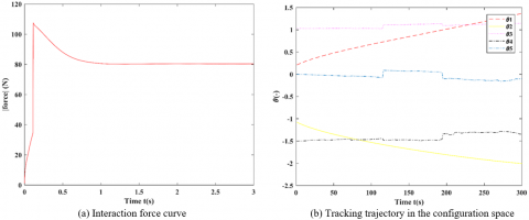
If the interaction force is known, it should be controlled by the strategy in Figure 9.
As shown in Figure 9, the interaction force rises abruptly in the early stage of motions, and then slowly drops, ending up in a stable state. Thus, the evolution of the interaction force can be divided into three phases: the rising phase, the decreasing phase and the stabilization phase. The control effect gradually improves, thanks to the adaptability of the control system in each phase.
As shown in Figure 9(b), the planned trajectory ensures the normal operation of the end effector, which outputs a relatively constant force as the manipulator moves. Therefore, the control process covers two aspects: the tracking of the angular displacement in the configuration space, and the tracking the force in cartesian space.
Figure 9. The control strategy for the case of known interaction force
4.1 Numerical tests
The desired trajectory was derived from the control law (31) and the parameter adaptation law. The simulation parameters are provided in Table 1. In addition, the adaptive gain matrix $\Gamma$ of the parameters can be set up as:
$\Gamma=\left[\begin{array}{llllll}{0.05} & {0.05} & {0.05} & {0.05} & {0.05} & {0.05}\end{array}\right]$.
Numerical tests were carried out under different scenarios, based on whether the interaction force is known and the modification of the control law. If the interaction force is known, the influence of the interaction force on the control system was assumed as Fin. Then, the control law was modified to ensure that the displacement and force errors converge to the boundary. The matrix $\Gamma$ can be expressed as:
$\mathrm{K}_{\mathrm{d}}=\operatorname{diag}[10 \quad 10 \quad 10 \quad 10 \quad 10]$
$\Lambda=\operatorname{diag}\left[\begin{array}{ccccc}{5} & {5} & {5} & {5} & {5}\end{array}\right]$
The initial values of the adaptive parameters can be presented as:
$\mathrm{\varsigma}_{0}(0)=0.015$
$\mathrm{\varsigma}_{1}(0)=0.015$
If the interaction force is unknown, the force was taken as the interference Fin in the system description. Then, the matrix $\Gamma$ can be expressed as:
$\Gamma=\operatorname{diag}[0.015 \quad 0.015 \quad 0.015 \quad 0.015 \quad 0.015 \quad 0.015]$
$\Lambda=\operatorname{diag}\left[\begin{array}{ccccc}{5} & {5} & {5} & {5} & {5}\end{array}\right]$.
The initial values of the adaptive parameters can be presented as:
$\mathrm{\varsigma}_{0}(0)=0.015$,
$\mathrm{\varsigma}_{1}(0)=0.015$.
$\text { In addition, } \eta_{1}(0)=0.8 \quad, \quad \eta_{2}(0)=0.2 \quad, \quad \eta_{3}(0)=$$0.2, \eta_{4}(0)=0.8, \eta_{5}(0)=0.8, \eta_{6}(0)=0.8, \sigma_{0}(0)=0$ and$\sigma_{1}(0)=0$.
4.2 Numerical results
This subsection provides the numerical results in both cases of the interaction force. Each simulation test lasted 3s, during which the input force fluctuated greatly.
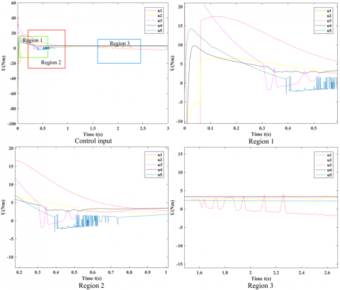
The total control signal is controlled by the adaptive model (Figure 10). The adaptive controller starts the compensation control (Region 1) at around 0.1s. The control signal tended to be smooth due to the parameter adaptation and the effect of sliding mode control (Region 2). In the initial phase of the manipulator motion, the compensation control was mismatched because the precise control parameters were unknown. At the beginning, the signal generated by proportional module had the dominance. Soon, the dominance was gradually weakened, while the parameter adaptation compensated for the control (Region 3).
The parameters were initially compensated by the proportional module, and the control parameters fluctuated about a certain value (Figure 11).
Figure 10. The total control signals in the case of known interaction force
Figure 11. Parameter adaptation in the case of known interaction force
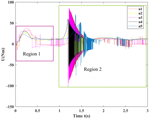
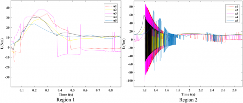
Figure 12 presents the numerical results in the case that both interaction force and interference were unknown. For trajectory smoothness, the sliding mode adaptive control was implemented. The time lag induced by the sliding mode structure makes the controller impossible to eliminate nonlinear fluctuations.
In the case of unknown interaction force, the sliding mode control $\widehat{\sigma}_{0} \mathrm{s}+\widehat{\sigma}_{1} \operatorname{sgn}(\mathrm{s})$ was adopted to ensure the robustness of the control system. As shown in Figure 13, the error function converged on the sliding surface, providing a guarantee to the smoothness of the trajectory error in the configuration space.
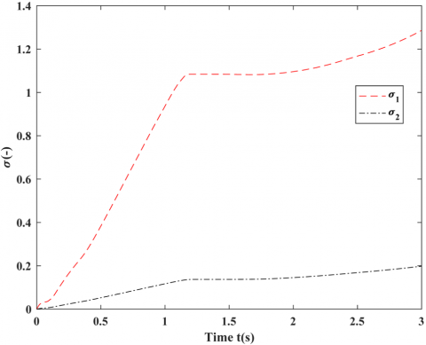
In the case of unknown interaction force, the estimated parameters presented a worst-case scenario with significant fluctuations in parameter values. As shown in Figures 14 and 15, the estimated system parameters were all bounded and eventually stabilized, indicating that our control system tended to be stable.
Figure 12. Control input of unknown input force in cartesian space
Figure 13. Control input of unknown input force in configuration space
Figure 14. Parameter adaptation in the case of unknown interaction force in cartesian space
In the case of unknown interaction force, the estimated parameters presented a worst-case scenario with significant fluctuations in parameter values. As shown in Figures 14 and 15, the estimated system parameters were all bounded and eventually stabilized, indicating that our control system tended to be stable.
Figure 15. Parameter adaptation in the case of unknown interaction force in configuration space
4.3 Discussion
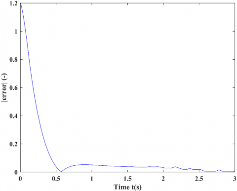
As shown in Figure 16(a), the error peak appeared in the initial phase, for the parameter adaptation law does not take effect. Then, the error plunged deeply over the time. Similarly, the force error curve (Figure 16(b)) was high at the beginning, because the adaptive law does not take effect, and later fluctuated and declined.
(a)
(b)
Figure 16. The joint angular error and interaction force error in the case of known interaction force
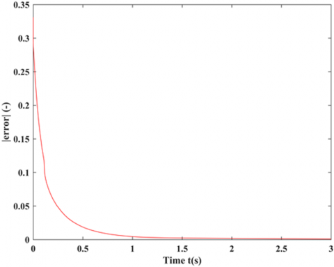
Figure 17 provides the interaction tracking error and the parameter estimation error in the case of unknown interaction force. It can be seen that both errors tended to land on the determined boundary. This confirms the stability of our control system.
For the error in the case of unknown interaction force, since the estimated term $\widehat{\sigma}_{0} \mathrm{s}+\widehat{\sigma}_{1} \operatorname{sgn}(\mathrm{s})$ begins to take effect, the error converged sharply, and slowly approached the equilibrium level. Thus, the adaptive control can clearly improve the control quality.
For the error in the case of known interaction force, the proportional module improved the initial control quality. To eliminate the error of the force control and position control, the parameter adaptation helps to enhance the control quality in the initial phase.
In both cases, the proportional module and the sliding mode module play a leading role in the early phase. In the later phase, the parameter adaptation evolves stably, improving the control quality. Finally, the adaptive control tracks the change trajectory of the force and position well, leading to the convergence of the force/position error.
Figure 17. The error in the case of known interaction force
This paper proposes a control method applicable to robots with varied load constraints and any DOF. Firstly, the nodal displacement of the manipulator was calculated by a full rank or rank deficient cartesian stiffness matrix. Then, the dynamics model of the manipulator was presented as a set of matrix equations by the Lagrange’s method in high-dimensional configuration space. This approach has a unique advantage: the model can be generated directly by aggregating the joint energy equation, without needing the global stiffness matrix.
Based on the dynamics model of flexible manipulator, a separate control strategy was developed to control the motions with known or unknown interaction force. After that, an adaptive controller was mathematically deduced, under the design principles of the control system under different conditions. The behavior of the control system was analyzed under the cases of known or unknown interaction force, and its stability was proved. The tracking error of the interaction force can converge through the parameter adaptation, under the Lyapunov’s principle.
Several numerical tests were conducted under different conditions of the interaction force, aiming to verify the effectiveness and superiority of our control strategy. The numerical results show that the sliding mode control is more stable and interference resistant than the adaptive control. However, due to the switching function, the sliding mode control cannot avoid the nonlinear fluctuations of the input, which undermines the motion control. Therefore, an accurate observer should be introduced to the control system to enhance the control effect for relatively stable input. In the case of known interaction force, the proportional module may compensate controlling quality in the initial phase of adaptive control. In the case of unknown interaction force, the position error will fluctuate during the convergence, but the control system remains stable.
This work is supported primarily by the National Key R&D Program of China (No. 2017YFC0806300), the National Key R&D Program of China (No. 2017YFC0806608).
[1] Tanaka, M., Tadakuma, K., Nakajima, M., Fujita, M. (2018). Task-space control of articulated mobile robots with a soft gripper for operations. IEEE Transactions on Robotics, 35(1): 135-146. http://dx.doi.org/10.1109/TRO.2018.2878361
[2] Leboutet, Q., Dean-Leon, E., Bergner, F., Cheng, G. (2019). Tactile-based whole-body compliance with force propagation for mobile manipulators. IEEE Transactions on Robotics, 35(2): 330-342. http://dx.doi.org/10.1109/TRO.2018.2889261
[3] Tanner, H.G. (2006). Mobile manipulation of flexible objects under deformation constraints. IEEE Transactions on Robotics, 22(1): 179-184. http://dx.doi.org/10.1109/TRO.2005.861452
[4] Giusti, A., Malzahn, J., Tsagarakis, N.G., Althoff, M. (2018). On the combined inverse-dynamics/passivity-based control of elastic-joint robots. IEEE Transactions on Robotics, 34(6): 1461-1471. http://dx.doi.org/10.1109/TRO.2018.2861917
[5] Hosseini-Pishrobat, M., Keighobadi, J. (2019). Robust vibration control and angular velocity estimation of a single-axis MEMS gyroscope using perturbation compensation. Journal of Intelligent & Robotic Systems, 94(1): 61-79. https://doi.org/10.1007/s10846-018-0789-5
[6] Katsura, S., Ohnishi, K. (2007). Force servoing by flexible manipulator based on resonance ratio control. IEEE Transactions on Industrial Electronics, 54(1): 539-547. http://dx.doi.org/10.1109/TIE.2006.888805
[7] Zhu, W.H. (2005). On adaptive synchronization control of coordinated multirobots with flexible/rigid constraints. IEEE Transactions on Robotics, 21(3): 520-525. http://dx.doi.org/10.1109/TRO.2004.839219
[8] Yu, Y.Q., Du, Z.C., Yang, J.X., Li, Y. (2011). An experimental study on the dynamics of a 3-rrr flexible parallel robot. IEEE Transactions on Robotics, 27(5): 992-997. http://dx.doi.org/10.1109/TRO.2011.2159408
[9] Renda, F., Boyer, F., Dias, J., Seneviratne, L. (2018). Discrete cosserat approach for multisection soft manipulator dynamics. IEEE Transactions on Robotics, 34(6): 1518-1533. http://dx.doi.org/10.1109/TRO.2018.2868815
[10] Liang, X., Huang, X., Wang, M., Zeng, X. (2010). Adaptive task-space tracking control of robots without task-space- and joint-space-velocity measurements. IEEE Transactions on Robotics, 26(4): 733-742. http://dx.doi.org/10.1109/TRO.2010.2051594
[11] Schill, M.M., Buss, M. (2018). Robust ballistic catching: A hybrid system stabilization problem. IEEE Transactions on Robotics, 34(6): 1502-1517. http://dx.doi.org/10.1109/TRO.2018.2868857
[12] Ulrich, S., Sasiadek, J.Z., Barkana, I. (2012). Modeling and direct adaptive control of a flexible-joint manipulator. Journal of Guidance, Control, and Dynamics, 35(1): 25-39. https://doi.org/10.2514/1.54083
[13] Serra, D., Ruggiero, F., Donaire, A., Buonocore, L.R., Lippiello, V., Siciliano, B. (2019). Control of nonprehensile planar rolling manipulation: A passivity-based approach. IEEE Transactions on Robotics, 35(2): 317-329. http://dx.doi.org/10.1109/TRO.2018.2887356
[14] Walsh, A., Forbes, J.R. (2015). Modeling and control of flexible telescoping manipulators. IEEE Transactions on Robotics, 31(4): 936-947. http://dx.doi.org/10.1109/TRO.2015.2441473
[15] Gueaieb, W., Al-Sharhan, S., Bolic, M. (2007). Robust computationally efficient control of cooperative closed-chain manipulators with uncertain dynamics. Automatica, 43(5): 842-851. http://dx.doi.org/10.1016/j.automatica.2006.10.025
[16] Roy, B., Asada, H.H. (2006). Dynamics and control of a gravity-assisted underactuated robot arm for assembly operations inside an aircraft wing-box. Proceedings 2006 IEEE International Conference on Robotics and Automation, 2006. ICRA 2006, pp. 701-706. http://dx.doi.org/10.1109/ROBOT.2006.1641792
[17] Kim, M.J., Chung, W.K. (2015). Disturbance-observer-based PD control of flexible joint robots for asymptotic convergence. IEEE Transactions on Robotics, 31(6): 1508-1516. http://dx.doi.org/10.1109/TRO.2015.2477957
[18] Dadfarnia, M., Jalili, N., Liu, Z., Dawson, D.M. (2004). An observer-based piezoelectric control of flexible cartesian robot arms: theory and experiment. Control Engineering Practice, 12(8): 1041-1053. https://doi.org/10.1016/j.conengprac.2003.09.003
[19] Magrini, E., Flacco, F., Luca, A.D. (2015). Control of generalized contact motion and force in physical human-robot interaction. 2015 IEEE International Conference on Robotics and Automation (ICRA), pp. 2298-2304. http://dx.doi.org/10.1109/ICRA.2015.7139504
[20] Gierlak, P., Szuster, M. (2017). Adaptive position/force control for robot manipulator in contact with a flexible environment. Robotics and Autonomous Systems, 95: 80-101. https://doi.org/10.1016/j.robot.2017.05.015