Mohamed Z. Fadel* | Mahmoud G. Rabie | Ahmed M. Youssef
OPEN ACCESS
The Fly-By-Wire (FBW) system is a computer-based flight control system that replaces the mechanical link between the pilot’s cockpit controls and the moving surfaces by much lighter electrical wires. This concept is applied in the electro-hydraulic servo systems. In the present work, a detailed non-linear mathematical model of an aircraft integrated servo actuator (ISA) is developed and a computer simulation program is built using MATLAB / SIMULINK package. The ISA mainly consists of two separate active hydraulic power systems, used to supply the ISA with the required power. The studied ISA incorporates two electro-hydraulic servo-valves, a twin-symmetrical-hydraulic actuating cylinder, and a smart design of built-in directional control valves with a feedback system. The output linear motion of the actuating cylinder of the ISA is presented and its transient response is analyzed. A classical PID and modified PI-D controllers are designed and tuned by Zeigler-Nichols method according to the Integral Square Error (ISE) criteria to minimize the difference between the obtained system output feedback and the desired set input by adjusting the system control parameters. The comparative study between the two types of controllers show that the modified PI-D controller has better response than basic one and slower in the presence of disturbance.
fly-by-wire system (FBW), integrated servo actuator (ISA), servo, actuating cylinder, PID controller, modified PI-D controller, integral squared error (ISE)
Fly-By-Wire (FBW) control system technology has greatly enhanced the flexibility of the parameters in airplanes design. This control systems provide a new interface for controlling airplane using digital technology to replace mechanical components. This system has enabled the development of a variety of innovative airplanes designs from aerodynamically unstable airplane to autonomous air vehicles. The digital computer-based system was able to provide improved maneuverability and weight reduction in both military and commercial applications at the cost of reduced reliability [1]. This concept is used in the electro-hydraulic servo systems, which have the functions of electric and hydraulic systems.
The electro-hydraulic servo systems play an important role in industrial applications, especially in flight simulators and actuating systems of the aircraft. The main reason of using hydraulic systems in many applications is that, they can provide a high torque and high force. In addition, the electric systems produce a high controllability and precision actuating motion. So, these systems are used to control the position of the maneuvering surfaces of the airplanes.
The electro-hydraulic servo system refers to the control system which combined two control modes of electrical and hydraulic. Transmitting the signal by use of electronic and electric parts, driving the load with hydraulic transmission in the electrohydraulic servo control system. So it can use an electrical system for its efficiency and suitability, and use of hydraulic system for its rapid response speed, big load stiffness and accurate positioning characteristics to make the whole system more adaptable [2].
Generally, the main objective of controlling the aircraft means to direct its orientation (attitudes) during its flight path according to the command motions with respect to the inertial or reference frame. To achieve this goal, controller is used. The most common controller is the proportional-integral-derivative (PID) controller. PID controller is the most common controller class of feedback systems. It is widely used in industrial control fields as stated by [3] and [4]. It has been used to minimize the difference between the measured system output feedback and the desired input by adjusting the system control parameters [5].
Many techniques have been developed for optimally tuning the controller’s parameters. These range from trial and error [6], root locus [7] and artificial intelligence techniques [8]. The performance indices, which are usually used in the optimization are integral absolute error (IAE), Integral Square Error (ISE) and Integral Time Absolute Error (ITAE) [9].
PID controller is one of the earliest developed control strategies. The design algorithm and control structure involved in PID controller are simple, and are suitable for engineering application background. Also, PID control scheme does not require accurate mathematical model of controlled object, and the control effect of PID control is commonly satisfactory. So PID controller in industry is one of the most widely used control strategies, and is more successful. According to statistics, PID controller applied to more than 90% in the industrial control of the controller [10].
In parallel PID controllers the reference input might contain a step component in which case the pure derivative term in the control action, produce an impulse function (delta function), such a phenomenon is called set-point kick. To overcome this phenomenon a pre-filter is used in the derivative term, or by using modified forms of PID control where the derivative action is only applied to the feedback path so that differentiation occurs only on the feedback signal and not on the reference signal [11].
In the present work, the output linear motion of the actuating cylinder of the ISA is presented and controlled by obtaining the transient response of the ISA. A classical PID and modified PI-D controllers are designed and tuned by Zeigler-Nichols method according to the Integral Square Error (ISE) criteria to minimize the difference between the obtained system output feedback and the desired set input by adjusting the system control parameters. A comparative study between the two controllers is performed.
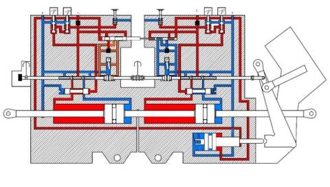
The studied system is an Integrated Servo Actuator (ISA) of an aircraft which incorporates two electro-hydraulic servo-valves (EHSV) and a smart design of four built-in direct operated directional control valves (DCV) controlled by four electrical solenoids and a switching DCV works as ON-OFF switch of the EHSV and a twin-symmetrical-hydraulic actuating cylinder with a feedback system as shown in Figure 1. The definitions and the numerical values of the overall model equations are collected and tabulated in Appendix-A.
Figure 1. ISA scheme
The dynamic behavior of the ISA system is described by a set of mathematical relations. Due to this complicated system, there are some assumptions are taken into consideration in the model [12]:
The ISA is divided into three modules; first, the pre-servovalve (SV) module, electro-hydraulic servovalve module, and the actuating hydraulic cylinder module. The mathematical relations that describe the system are deduced as follow:
2.1 Pre-servovalve module
This part of the ISA is consisting generally of a smart design of built-in direct operated directional control valves (DCV), controlled by electrical solenoids.
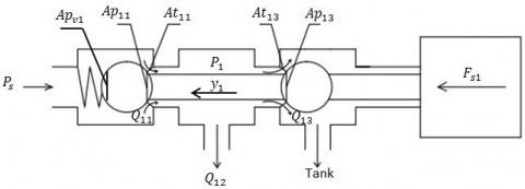
2.1.1 Single direct operated DCV
Figure 2. Single DCV operational scheme
Equation of motion
By energizing the electric solenoid, the solenoid force ( Fs1) acts on the moving parts against the pressure forces, spring forces, seat reaction forces, viscous friction forces and inertia forces as shown in Figure 2. The motion during this mode is described by the following relations:
$\mathbf { F } _ { \mathbf { S } _ { \mathbf { 1 } } } = \mathbf { m } \ddot { \mathbf { y } } _ { \mathbf { 1 } } + \mathbf { f } _ { \mathbf { v } } \dot { \mathbf { y } } _ { \mathbf { 1 } } + \mathbf { K } _ { \mathbf { s p } } \left( \mathbf { y } _ { \mathbf { o } } + \mathbf { y } _ { \mathbf { 1 } } \right) + \mathbf { P } _ { \mathbf { S } \mathbf { 1 } } \mathbf { A } \mathbf { p } _ { \mathbf { v } 1 } - \mathbf { P } _ { \mathbf { 1 } } \mathbf { A } \mathbf { p } _ { \mathbf { 1 1 } } +$ $\mathbf { P } _ { \mathbf { 1 } } \mathbf { A } \mathbf { p } _ { 1 \mathbf { 3 } } - \mathbf { F } _ { \mathbf { S R } \mathbf { 1 } }$ (1)
Seat reaction force
The poppet’s displacement in the closure direction is limited mechanically. When reaching its seat, a seat reaction force takes place due to the action of the structural damping of the seat material.
$\mathrm { F } _ { \mathrm { SR } 1 } = \mathrm { F } _ { 1 \mathrm { L } } - \mathrm { F } _ { 1 \mathrm { R } }$ (2)
$\mathrm { F } _ { 1 \mathrm { L } } = \left\{ \begin{array} { l l } { 0 } & { \mathrm { y } _ { 1 } > 0 } \\ { - \mathrm { K } _ { \mathrm { sm } } \mathrm { y } _ { 1 } - \mathrm { f } _ { \mathrm { sm } } \dot { \mathrm { y } } _ { 1 } } & { \mathrm { y } _ { 1 } \leq 0 } \end{array} \right.$ (3)
$\mathrm { F } _ { 1 \mathrm { R } } = \left\{ \begin{array} { l l } { 0 } & { \mathrm { y } _ { 1 } < \mathrm { y } _ { \mathrm { i } } } \\ { \mathrm { K } _ { \mathrm { sm } } \left( \mathrm { y } _ { 1 } - \mathrm { y } _ { \mathrm { i } } \right) + \mathrm { f } _ { \mathrm { sm } } \dot { \mathrm { y } } _ { 1 } } & { \mathrm { y } _ { 1 } \geq \mathrm { y } _ { \mathrm { i } } } \end{array} \right.$ (4)
Flow rates through the throttling areas
There are two flow rates through the two throttling areas $\mathrm { At } _ { 11 }$ and $\mathrm { At } _ { 13 }$. These flow rates are given by the following expressions:
$\mathrm { Q } _ { 11 } = \mathrm { C } _ { \mathrm { d } } \mathrm { At } _ { 11 } \sqrt { \frac { 2 \left( \mathrm { P } _ { \mathrm { S } 1 } - \mathrm { P } _ { 1 } \right) } { \rho } }$ (5)
$\mathrm { Q } _ { 13 } = \mathrm { C } _ { \mathrm { d } } \mathrm { At } _ { 13 } \sqrt { \frac { 2 \left( \mathrm { P } _ { 1 } - \mathrm { P } _ { \mathrm { t } } \right) } { \rho } }$ (6)
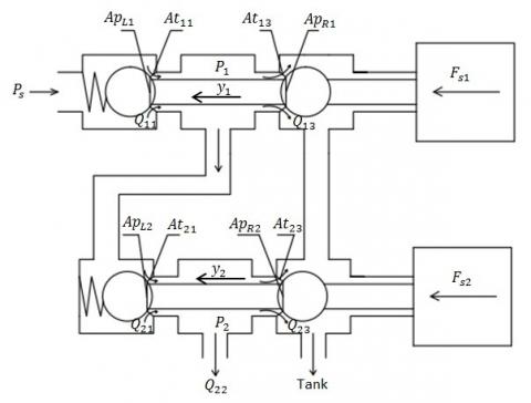
2.1.2 Combined direct operated DCV
The first and second DCV’s is the same structure and will form the combined direct operated DCV. This configuration is considered to be in the main and secondary ISA system, Figure 1.
Figure 3. Combined DCV operational scheme
Equation of motion
The motion of this combined DCV, Figure 3 is described by the following relation:
$\mathbf { F } _ { \mathrm { S } 2 } = \mathbf { m } \ddot { y } _ { 2 } + \mathbf { f } _ { \mathbf { v } } \dot { \mathbf { y } } _ { 2 } + \mathbf { K } _ { \mathrm { sp } } \left( \mathbf { y } _ { \mathrm { o } } + \mathbf { y } _ { 2 } \right) + \mathbf { P } _ { 1 } \mathbf { A } \mathbf { p } _ { \mathbf { v } 2 } - \mathbf { P } _ { 2 } \mathbf { A } \mathbf { p } _ { 2 \mathbf { 1 } } +$ $\mathbf { P } _ { 2 } \mathbf { A } \mathbf { p } _ { 23 } - \mathbf { F } _ { \mathrm { SR } 2 }$ (7)
Seat reaction force
The poppet’s displacement in the closure direction is limited mechanically. When reaching its seat, a seat reaction force takes place due to the action of the structural damping of the seat material.
$\mathrm { F } _ { \mathrm { SR } 2 } = \mathrm { F } _ { 2 \mathrm { L } } - \mathrm { F } _ { 2 \mathrm { R } }$ (8)
$\mathrm { F } _ { 2 \mathrm { L } } = \left\{ \begin{array} { l l } { 0 } & { \mathrm { y } _ { 2 } > 0 } \\ { - \mathrm { f } _ { \mathrm { sm } } \dot { \mathrm { y } } _ { 2 } - \mathrm { K } _ { \mathrm { sm } } \mathrm { y } _ { 2 } } & { \mathrm { y } _ { 2 } \leq 0 } \end{array} \right.$ (9)
$\mathrm { F } _ { 2 \mathrm { R } } = \left\{ \begin{array} { l l } { 0 } & { \mathrm { y } _ { 2 } < \mathrm { y } _ { \mathrm { i } } } \\ { \mathrm { f } _ { \mathrm { sm } } \dot { \mathrm { y } } _ { 2 } + \mathrm { K } _ { \mathrm { sm } } \left( \mathrm { y } _ { 2 } - \mathrm { y } _ { \mathrm { i } } \right) } & { \mathrm { y } _ { 2 } \geq \mathrm { y } _ { \mathrm { i } } } \end{array} \right.$ (10)
Flow rates through the throttling areas
There are two flow rates through the two throttling areas $\mathrm { At } _ { 21 }$ and $\mathrm { At } _ { 23 }$ Figure 3. These flow rates are given by the following expressions:
$\mathrm { Q } _ { 21 } = \mathrm { C } _ { \mathrm { d } } \mathrm { At } _ { 21 } \sqrt { \frac { 2 \left( \mathrm { P } _ { 1 } - \mathrm { P } _ { 2 } \right) } { \rho } }$ (11)
$\mathrm { Q } _ { 23 } = \mathrm { C } _ { \mathrm { d } } \mathrm { At } _ { 23 } \sqrt { \frac { 2 \left( \mathrm { P } _ { 2 } - \mathrm { P } _ { \mathrm { t } } \right) } { \rho } }$ (12)
Continuity equation of the valve chamber
There are two chambers (a) and (b) as shown in Figure 3. The first chamber (a) is connecting the first and second valve together. The inlet flow rates of chamber (a) are Q11 and Q12, while the output is Q13. The continuity equation of the valve chamber (a) is:
$\mathbf { Q } _ { 11 } - \mathbf { Q } _ { 13 } - \mathbf { Q } _ { 21 } = \frac { \mathbf { v } _ { 1 } } { \mathbf { B } } \frac { \mathrm { d } \mathbf { P } _ { 1 } } { \mathrm { dt } }$ (13)
2.1.3 Switching DCV
The switching DCV is displaced by the pressure forces, controlled by the direct operated DCV. The switching DCV is treated as (ON-OFF) switch for the main and secondary systems of the EHSV as shown in Figure 4.
Figure 4. Single DCV operational scheme
Equation of motion
Its motion is described by this relation:
$\mathbf { P } _ { 2 } \mathbf { A } _ { \mathbf { p L } } - \mathbf { P } _ { \mathbf { s } 1 } \mathbf { A } _ { \mathbf { r L } } + \mathbf { P } _ { s 2 } \mathbf { A } _ { \mathbf { r R } } - \mathbf { P } _ { \mathbf { 4 } } \mathbf { A } _ { \mathbf { p R } } - \mathbf { F } _ { \mathbf { S R S } }$ $= \mathbf { m } _ { 5 } \ddot { \mathbf { y } } _ { \mathbf { 5 } } + \mathbf { f } _ { 5 } \mathbf { y } _ { 5 }$ (14)
Seat reaction force
There are four seat reaction forces effect on the SDCV ($\mathrm { F } _ { 5 \mathrm { L } 1 } , \mathrm { F } _ { 5 \mathrm { R } 1 } , \mathrm { F } _ { 5 \mathrm { L } 2 }$ and $\mathrm { F } _ { 5 \mathrm { R } 2 }$) as shown in Figure 4.
$\mathrm { F } _ { \mathrm { SR } 5 } = \mathrm { F } _ { 5 \mathrm { R } 1 } + \mathrm { F } _ { 5 \mathrm { R } 2 } - \mathrm { F } _ { 5 \mathrm { L } 1 } - \mathrm { F } _ { 5 \mathrm { L } 2 }$
(15)
$\mathrm { F } _ { 5 \mathrm { R } 1 } = \mathrm { F } _ { 5 \mathrm { R } 2 } = \left\{ \begin{array} { l l } { ^ { \mathrm { f } _ { \mathrm { sm } } } \dot{\mathrm { y } _ { 5 }} + \mathrm { K } _ { \mathrm { sm } } \left( \mathrm { y } _ { 5 } - \mathrm { y } _ { \mathrm { siR } } \right) } & { \mathrm { y } _ { 5 } \geq \mathrm { y } _ { \mathrm { siR } } } \\ { 0 } & { \mathrm { y } _ { 5 } < \mathrm { y } _ { \mathrm { siR } } } \end{array} \right.$ (16)
$\mathrm { F } _ { 5 \mathrm { L } 1 } = \mathrm { F } _ { 5 \mathrm { L } 22 } = \left\{ \begin{array} { l l } { - \mathrm { f } _ { \mathrm { sm } } \dot{\mathrm { y } _ { 5 }} - \mathrm { K } _ { \mathrm { sm } } \left( \mathrm { y } _ { 5 } - \mathrm { y } _ { 5 \mathrm { iL } } \right) } & { \mathrm { y } _ { 5 } \leq \mathrm { y } _ { 5 \mathrm { iL } } } \\ { 0 } & { \mathrm { y } _ { 5 } > \mathrm { y } _ { 5 \mathrm { il } } } \end{array} \right.$ (17)
Continuity equation of the switching DCV chambers
The switching DCV has two chambers in the right and left sides. The left chamber is connected to the second DCV (room b) that has exit pressure P2, but the right chamber is connected to the fourth DCV that has exit pressure P4. Neglecting the internal leakage and the external leakage, the continuity equations of the valve chambers will be:
$\mathrm { Q } _ { 21 } - \mathrm { Q } _ { 23 } - \mathrm { A } _ { \mathrm { PL } } \dot{\mathrm { y } _ { 5 }} = \frac { \mathrm { v } _ { 2 } + \mathrm { A } _ { \mathrm { PL } } \mathrm { Y } _ { 5 } } { \mathrm { B } } \frac { \mathrm { dP } _ { 2 } } { \mathrm { dt } }$ (18)
$\mathrm { Q } _ { 41 } - \mathrm { Q } _ { 43 } + \mathrm { A } _ { \mathrm { PR } } \dot{\mathrm { y } _ { 5 }} = \frac { \mathrm { v } _ { 4 } - \mathrm { A } _ { \mathrm { PR } } \mathrm { y } _ { 5 } } { \mathrm { B } } \frac { \mathrm { dP } _ { 4 } } { \mathrm { dt } }$ (19)
2.2 Electro-hydraulic servovalve module
This module contains mainly main and secondary two-stage EHSV’s which control the motion of the main driven spool valve. The mathematical model of the main EHSV is deduced completely.
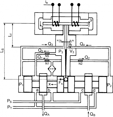
This model is describing the dynamic performance of a two-stage EHSV. The schematic two-stage EHSV is shown in Figure 5.
Figure 5. Two stage EHSV scheme
2.2.1 Electromagnetic torque motor
The electromagnetic torque motor converts an electric input signal of low-level current (usually within 10 mA) into a proportional mechanical torque. The motor is usually designed to be separately mountable, testable, interchangeable, and hermetically sealed against the hydraulic fluid. The net torque depends on the effective input current and the flapper rotational angle. Neglecting the effect of the magnetic hysteresis, the following expression for the torque can be deduced:
$\mathbf { T } = \mathbf { K } _ { \mathbf { i } } \mathbf { i } _ { \mathbf { e } } + \mathbf { K } _ { \boldsymbol { \theta } } \boldsymbol { \theta }$ (20)
2.2.2 Armature model
The motion of the rotating armature and attached elements is governed by the following equations:
Armature equation of motion
$\mathrm { T } = \mathrm { j } \ddot { \theta } + \mathrm { f } _ { \theta } \dot { \theta } + \mathrm { K } _ { \mathrm { T } } \theta + \mathrm { T } _ { \mathrm { L } } + \mathrm { T } _ { \mathrm { P } } + \mathrm { T } _ { \mathrm { F } }$ (21)
$\mathrm { T } _ { \mathrm { P } } = \frac { \pi } { 4 } \mathrm { d } _ { \mathrm { f } } ^ { 2 } \left( \mathrm { P } _ { 2 \mathrm { L } } - \mathrm { P } _ { 1 \mathrm { L } } \right) \mathrm { L } _ { \mathrm { f } }$ (22)
Feedback Torque
The feedback torque depends on the spool displacement and the flapper rotational angle as given by the following equations:
$\mathrm { T } _ { \mathrm { F } } = \mathrm { F } _ { \mathrm { s } } \mathrm { L } _ { \mathrm { s } }$ (23)
$\mathrm { F } _ { \mathrm { s } } = \mathrm { K } _ { \mathrm { s } } \left( \mathrm { L } _ { \mathrm { s } } \theta + \mathrm { x } \right)$ (24)
$\mathrm { T } _ { \mathrm { F } } = \mathrm { K } _ { \mathrm { s } } \mathrm { L } _ { \mathrm { s } } \left( \mathrm { L } _ { \mathrm { s } } \theta + \mathrm { x } \right)$ (25)
Flapper Position Limiter
The flapper displacement is limited mechanically by the jet nozzles. When reaching any of the side nozzles, the seat reaction develops a counter torque, given by the following equation:
$\mathrm { T } _ { \mathrm { L } } = \left\{ \begin{array} { l l } { 0 } & { \left| \mathrm { x } _ { \mathrm { f } } \right| < \mathrm { x } _ { \mathrm { i } } } \\ { \mathrm { R } _ { \mathrm { s } } \dot { \theta } - \left( \left| \mathrm { x } _ { \mathrm { f } } \right| - \mathrm { x } _ { \mathrm { i } } \right) \mathrm { K } _ { \mathrm { L } \mathrm { f } _ { \mathrm { f } } } \mathrm { L } _ { \mathrm { f } } } & { \left| \mathrm { x } _ { \mathrm { f } } \right| > \mathrm { x } _ { \mathrm { i } } } \end{array} \right.$ (26)
2.2.3 Restriction areas
The restriction areas in the switching DCV and in the flapper valve are shown in Figure 6 and given by the following relations:
Figure 6. Throttling areas and flow rates
$A _ { 0 } = \frac { \pi } { 4 } d _ { f } ^ { 2 }$ (27)
$A _ { 3 } = \pi d _ { f } \left( x _ { i } + x _ { f } \right)$ (28)
$\mathrm { A } _ { 4 } = \pi \mathrm { d } _ { \mathrm { f } } \left( \mathrm { x } _ { \mathrm { i } } - \mathrm { x } _ { \mathrm { f } } \right)$ (29)
$A _ { 5 } = \frac { \pi } { 4 } d _ { 5 } ^ { 2 }$ (30)
$A _ { t h } = \omega * \left| y _ { 5 } \right|$ (31)
$A _ { B p } = \omega * \left| d _ { i } - y _ { 5 } \right|$ (32)
$\mathrm { x } _ { \mathrm { f } } = \mathrm { L } _ { \mathrm { f } } \theta$ (33)
Flow rates through switching DCV and flapper valve restrictions
The flow rates through the switching DCV and the flapper valve restrictions are shown in Figure 6 and given by the following equations:
$\mathrm { Q } _ { 1 } = \mathrm { C } _ { \mathrm { d } } \mathrm { A } _ { 0 } \sqrt { \frac { 2 \left( \mathrm { P } _ { \mathrm { s } } - \mathrm { P } _ { 1 } \right) } { \rho } }$ (34)
$\mathrm { Q } _ { 2 } = \mathrm { C } _ { \mathrm { d } } \mathrm { A } _ { 0 } \sqrt { \frac { 2 \left( \mathrm { P } _ { \mathrm { s } } - \mathrm { P } _ { 2 } \right) } { \rho } }$ (35)
$\mathrm { Q } _ { 3 } = \mathrm { C } _ { \mathrm { d } } \mathrm { A } _ { 3 } \sqrt { \frac { 2 \left( \mathrm { P } _ { 1 } - \mathrm { P } _ { 3 } \right) } { \rho } }$ (36)
$\mathrm { Q } _ { 3 } = \mathrm { C } _ { \mathrm { d } } \mathrm { A } _ { 3 } \sqrt { \frac { 2 \left( \mathrm { P } _ { 1 } - \mathrm { P } _ { 3 } \right) } { \rho } }$ (37)
$\mathrm { Q } _ { 5 } = \mathrm { C } _ { \mathrm { d } } \mathrm { A } _ { 5 } \sqrt { \frac { 2 \left( \mathrm { P } _ { 3 } - \mathrm { P } _ { \mathrm { t } } \right) } { \rho } }$ (38)
$\mathrm { Q } _ { \mathrm { th } } = \mathrm { C } _ { \mathrm { d } } \mathrm { A } _ { \mathrm { th } } \sqrt { \frac { 2 \left( \mathrm { P } _ { \mathrm { s } 1 } - \mathrm { P } _ { \mathrm { s } } \right) } { \rho } }$ (39)
$\mathrm { Q } _ { \mathrm { Bp } } = \mathrm { C } _ { \mathrm { d } } \mathrm { A } _ { \mathrm { Bp } } \sqrt { \frac { 2 \left( \mathrm { P } _ { 2 } - \mathrm { P } _ { 1 } \right) } { \rho } }$ (40)
Continuity equations applied to flapper valve chambers
Applying the continuity equation to the flapper valve chambers (a, b, c, and d) respectively (see Figure 7) and neglecting the internal leakage and the external leakage, the following equations have been obtained:
$\mathrm { Q } _ { 1 } + \mathrm { Q } _ { \mathrm { Bp } } - \mathrm { Q } _ { 3 } + \mathrm { A } _ { \mathrm { s } } \dot { \mathrm { x } } = \frac { \mathrm { v } _ { 0 } - \mathrm { A } _ { \mathrm { s } } \mathrm { x } } { \mathrm { B } } \frac { \mathrm { dP } _ { 1 } } { \mathrm { dt } }$ (41)
$\mathrm { Q } _ { 2 } - \mathrm { Q } _ { \mathrm { Bp } } - \mathrm { Q } _ { 4 } - \mathrm { A } _ { \mathrm { s } } \dot { \mathrm { x } } = \frac { \mathrm { v } _ { 0 } + \mathrm { A } _ { \mathrm { s } } \mathrm { x } } { \mathrm { B } } \frac { \mathrm { dP } _ { 2 } } { \mathrm { dt } }$ (42)
$\mathrm { Q } _ { 3 } + \mathrm { Q } _ { 4 } - \mathrm { Q } _ { 5 } = \frac { \mathrm { V } _ { 3 } } { \mathrm { B } } \frac { \mathrm { dP } _ { 3 } } { \mathrm { dt } }$ (43)
$\mathrm { Q } _ { \mathrm { th } } - \mathrm { Q } _ { 1 } - \mathrm { Q } _ { 2 } = \frac { \mathrm { v } _ { \mathrm { L } } } { \mathrm { B } } \frac { \mathrm { d } \mathrm { P } _ { \mathrm { sL } } } { \mathrm { dt } }$ (44)
Figure 7. Flapper valve chambers
2.2.4 Equation of motion of the spool
The motion of the spool valve is produced from the difference in pressure forces which act against seat reaction forces, viscous friction forces and inertia forces in the main and secondary EHSV’s. The mathematical model of the main EHSV is deduced above in detail. For the secondary EHSV, its mathematical model is deduced by the same manner. The equation of motion of the main driven spool valve is described by:
$\left( P 2 _ { L } - P 1 _ { L } \right) A _ { s } + \left( P 2 _ { R } - P 1 _ { R } \right) A _ { s } = m _ { s } \ddot { x } + f _ { s } \dot { x } +$ $K _ { s } L _ { s } \theta _ { L } + K _ { s } L _ { s } \theta _ { R } + 2 K _ { s } x$ (45)
2.3 Actuating hydraulic cylinder module
This module consists of two typical interconnection valves and a twin-symmetrical-hydraulic actuating cylinder with a feedback system as shown in Figure 8. The detailed mathematical modelling of this module is deduced as follow
Figure 8. Actuating cylinder module
2.3.1 Interconnection valve model
Equation of motion
The motion of this valve is described by this equation of motion. This valve works as a by-pass valve.
$\mathrm { P } _ { \mathrm { s } 1 } \mathrm { A } _ { \mathrm { Pz } } = \mathrm { m } _ { \mathrm { z } } \ddot { \mathrm { z } } + \mathrm { f } _ { \mathrm { z } } \dot { \mathrm { z } } + \mathrm { K } _ { \mathrm { sp } } \left( \mathrm { z } - \mathrm { z } _ { 0 } \right) - \mathrm { F } _ { \mathrm { sR } }$ (46)
Seat reaction forces
$\mathrm { F } _ { \mathrm { SR } } = \left\{ \begin{array} { l l } { 0 } & { \mathrm { z } > 0 } \\ { - \mathrm { f } _ { \mathrm { sm } } * \dot { \mathrm { z } } - \mathrm { K } _ { \mathrm { sm } } * \mathrm { z } } & { \mathrm { z } \leq 0 } \end{array} \right.$ (47)
2.3.2 Actuating cylinder model
The actuating cylinder is a cylinder of twin symmetrical type as shown in Figure 9. Its motion is performed against the pressure, inertia, viscous, and the seat reaction forces which described by the following relations:
Figure 9. Actuating cylinder scheme
The restriction areas through the spool valve are described as follow (Figure 10):
Figure 10. Restriction areas
$\left.\begin{array} { l } { A _ { a } = A _ { c } = \omega c } \\ { A _ { b } = A _ { d } = \omega \sqrt { x ^ { 2 } + c ^ { 2 } } } \end{array} \right\}$ for $x \geq 0$ (48)
$\left.\begin{array} { l } { A _ { a } = A _ { c } = \omega \sqrt { x ^ { 2 } + c ^ { 2 } } } \\ { A _ { b } = A _ { d } = \omega c } \end{array} \right\}$ for $x \geq 0$ (49)
$A _ { B P } = \omega * \left| d _ { i } - z \right|$ (50)
Flow rates through the spool valve
The rates through the restriction areas of the spool valve are described as follow:
$Q _ { a } = C _ { d } A _ { a } \sqrt { \frac { 2 \left( P _ { A } - P _ { t } \right) } { \rho } }$ (51)
$Q _ { b } = C _ { d } A _ { b } \sqrt { \frac { 2 \left( P _ { s 1 } - P _ { A } \right) } { \rho } }$ (52)
$Q _ { c } = C _ { d } A _ { c } \sqrt { \frac { 2 \left( P _ { s 1 } - P _ { B } \right) } { \rho } }$ (53)
$Q _ { d } = C _ { d } A _ { d } \sqrt { \frac { 2 \left( P _ { B } - P _ { t } \right) } { \rho } }$ (54)
$Q _ { a } = C _ { d } A _ { a } \sqrt { \frac { 2 \left( P _ { A } - P _ { t } \right) } { \rho } }$ (55)
$Q _ { B P } = C _ { d } A _ { B P } \sqrt { \frac { 2 \left( P _ { A } - P _ { B } \right) } { \rho } }$ (56)
Continuity equations applied to the cylinder chambers
The actuating cylinder has two chambers, (A and B). Neglecting the internal and external leakage.
The continuity equations of each chamber are described as follows:
$Q _ { b } - Q _ { a } - Q _ { B P } - A _ { p } \dot { y } = \frac { V _ { c } + A _ { p } y } { B } \frac { d P _ { A } } { d t }$ (57)
$Q _ { d } - Q _ { c } + Q _ { B P } + A _ { p } \dot { y } = \frac { V _ { c } - A _ { p } y } { B } \frac { d P _ { B } } { d t }$ (58)
Seat reaction forces
The piston displacement in the closure direction is limited mechanically. When reaching its seat, a seat reaction force takes place due to the action of the structural damping of the seat material.
There are four components of seat reaction force effects on the cylinder piston:
$F _ { S R C } = F _ { c R 1 } + F _ { c R 2 } - F _ { c L 1 } - F _ { c L 2 }$ (59)
$\mathrm { F } _ { \mathrm { cR } 1 } = \mathrm { F } _ { \mathrm { cR } 2 } = \left\{ \begin{array} { l l } { \mathrm { f } _ { \mathrm { sm } } \dot { \mathrm { y } } + \mathrm { K } _ { \mathrm { sm } } \left( \mathrm { y } - \mathrm { y } _ { \mathrm { ciR } } \right) } & { \mathrm { y } \geq \mathrm { y } _ { \mathrm { ciR } } } \\ { 0 } & { \mathrm { y } < \mathrm { y } _ { \mathrm { ciR } } } \end{array} \right.$ (60)
$\mathrm { F } _ { \mathrm { cL } 1 } = \mathrm { F } _ { \mathrm { cL } 2 } = \left\{ \begin{array} { c c } { - \mathrm { f } _ { \mathrm { sm } } \dot { \mathrm { y } } - \mathrm { K } _ { \mathrm { sm } } \left( \mathrm { y } + \mathrm { y } _ { \mathrm { ciL } } \right) } & { \left( \mathrm { y } + \mathrm { y } _ { \mathrm { ciL } } \right) \leq 0 } \\ { 0 } & { \left( \mathrm { y } + \mathrm { y } _ { \mathrm { ciL } } \right) > 0 } \end{array} \right.$ (61)
Equation of motion
The motion of the piston under the action of pressure, viscous friction, inertia, and external forces is described by the following equation, assuming unloaded piston:
$\left( \mathrm { P } _ { \mathrm { AL } } - \mathrm { P } _ { \mathrm { BL } } + \mathrm { P } _ { \mathrm { AR } } - \mathrm { P } _ { \mathrm { BR } } \right) \mathrm { A } _ { \mathrm { P } } = \mathrm { m } _ { \mathrm { P } } \ddot { \mathrm { y } } + \mathrm { f } _ { \mathrm { P } } \dot { \mathrm { y } } + \mathrm { K } _ { \mathrm { p } } \mathrm { y } + \mathrm { F } _ { \mathrm { SRC } }$ (62)
2.3.3 Feedback system
The piston displacement is picked up by a displacement transducer and feedback to the electronic controller, which generates the corresponding error signal.
The feedback loop can be described by the following equations:
$i _ { e } = i _ { c } - i _ { f }$ (63)
$i _ { f } = K _ { F B } \mathrm { y } $ (64)
PID controller consists of Proportional, Integral and Derivative action. PID controller algorithm is used in feedback loops and can be implemented in many forms. Classical PID controller has good static performance, simple designing technique, reliability and robustness [13]. Design and tuning of PID controllers have been large research areas ever since Ziegler and Nichols presented their methods in 1942. A standard PID controller is also known as “three-term” controller. The utilized PID controller is characterized by three parameters $K _ { p } , K _ { i }$ and $K _ { d }$ and the main task is to find the optimal values for these parameters according to the Integral Square Error (ISE) criteria, Figure 11.
Figure 11. PID controller
3.1 Classical PID controller design
The PID controller parameters are the proportional gain $K _ { p }$ , the integral gain $K _ { i }$ and the derivative gain $K _ { d }$ . The most well-known methods for estimating the PID parameters are those developed by Ziegler and Nichols method according to Table 1. They have had a major influence on the practice of the PID control for more than half a century. The general transfer function of the PID controller is:
$G _ { C } = K _ { P } + \frac { K _ { i } } { S } + K _ { d } S$ (65)
where, $K _ { P } = K , K _ { i } = \frac { K } { T _ { i } } , K _ { d } = K * T _ { d }$
Table 1. Ziegler-nichols first method rules for estimating the PID controller parameters [11]
|
Controller |
Symbol |
Gain K |
Ti[s] |
Td[s] |
|
Proportional |
P |
T/L |
- |
- |
|
Proportional integral |
PI |
0.9 T/L |
L/0.3 |
- |
|
Proportional integral derivative |
PID |
1.2 T/L |
2 L |
0.5 L |
Usually, the design of PID controller, based upon the first estimated parameters does not give satisfactory results. Therefore, a tuning process is recommended for each of the three PID controller parameters $K _ { p } , K _ { i }$ and $K _ { d }$. This tuning process aims to finding the optimum values of these parameters which minimize the steady state error according to ISE criteria. The PID with tuned parameters gives usually quite acceptable results.
The main objective is to tune the gains $K _ { p } , K _ { i }$ and $K _ { d }$ that can minimize the performance index according to ISE criteria. The equation of the performance index that used in this work is illustrated as follows [13]:
$I S E = \int _ { 0 } ^ { \infty } e ( t ) ^ { 2 } d t$ (66)
$e ( t ) = y _ { s s } - y ( t )$ (67)
where, $y _ { s s }$ the required steady state value, and $y ( t )$ is the actual response.
3.3 Modified PI-D controller
In parallel PID controllers the reference input might contain a step component in which case the pure derivative term in the control action, produce an impulse function (delta function), such a phenomenon is called set-point kick. To overcome this phenomenon a pre-filter is used in the derivative term, or by using modified forms of PID control where the derivative action is only applied to the feedback path so that differentiation occurs only on the feedback signal and not on the reference signal. The control scheme arranged in this way is called the PI-D controller. Figure 12a and 12b illustrate the structure of both types of controllers.
(a) PID controller structure
(b) Modified PI-D controller structure
Figure 12. PID controller structure and modified PI-D controller structure
3.4 Control system requirements
It should be clearly realized that the resulting control system, if properly designed, will give good time responses for any arbitrary reference command signal. The controllers are designed to meet the specifications of [14]:
Command tracking for unit step:
-Overshoot < 0.5 %
-Rise time < 1 sec
-Settling time < 5 sec
-Minimum steady state error ≈ zero
Disturbance rejection of about 90% within 1 sec.
The simulation program is built considering numerical values of a typical electro-hydraulic servo actuator (EHSA) which is stated in Appendix-A. Equations from (1) to (64) describe the dynamic performance and the transient response of the ISA system. These equations represent a detailed non-linear mathematical modeling of the system that used to develop a computer simulation program using MATLAB/SIMULINK package. This transient response is obtained by the simulation program to a 10 mA step input current with a step time of 2 second. The ISA system response is over-damped with a steady state value of 4 cm, a settling time of 6.51 second, and a rise time of 3.126 second, overshoot of 0.43 % and with steady state error of 0.00308 %. The transient response of the ISA is shown in Figure 13.
In order to achieve the control system requirements, a classical PID controller should be used. The values of the PID controller parameters are calculated using Zeigler-Nichols method. The tuning technique is applied to the system according to the ISE criteria for obtaining the minimum steady state error between the output feedback and the input current signal.
The tuned PID control parameters are $K _ { p } = 3.17 , K _ { i } =$ $- 0.0012$ and $K _ { d } = 0.293 .$ After applying the tuned $\mathrm { PID }$ controller in the system, the performance of the system is improved. Figure 14 shows the transient response of the ISA with the tuned PID control parameters.
Figure 13. Step response of the ISA without controller
Figure 14. Step response of the ISA with classical PID controller
In analyzing and designing control systems, the basis of performance comparison of various control systems is set up by specifying particular test input signals and by comparing the various systems responses to these input signals. The commonly used test input signals are step functions, ramp functions, acceleration functions, impulse-functions and sinusoidal functions.
To overcome the phenomena of set-point kick, the modified PI-D controller should be applied to the ISA system. This will be made by performing a trial and error method to optimize the values of the controller parameters that achieve the control system requirements. The modified PI-D controller parameters are obtained as follow, $K _ { p } = 4.53 , K _ { i } = 0.148$ and $K _ { d } = 0.284$. After applying these parameters in the system, the performance of the system is improved. Figure 15 shows the transient response of the ISA with the modified PI-D controller.
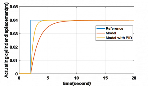
The controller is designed and tested for various operating points. Comparative synthesis of the ISA system controllers between PID and PI-D is performed. The transient response of the ISA system with classical PID and modified PI-D is shown in Figure 16.
To study the system behavior in the presence of disturbance, a disturbance signal shown in Figure 17 is applied to the system which arranged in the system as shown in Figure 18.
Figure 15. Step response of the ISA with modified PI-D controller
Figure 16. ISA response with PID and modified PI-D controllers
Figure 17. Applied disturbance signal
Figure 18. Disturbance signal arrangement
The transient response of the controlled ISA system in presence of disturbance is shown in Figure 19.
Figure 19. ISA response with pid and modified PI-D controllers in presenec of disturbance
Table 2 shows the values of the controller parameters and time response parameters with both controllers. Figure 20 shows the disturbance rejection for both controllers.
Figure 20. Disturbance reduction
Table 2. Controller design parameters
|
Control Parameters |
Model |
PID |
Modified PI-D |
|
kp |
0 |
3.17 |
4.53 |
|
ki |
0 |
-0.0012 |
0.148 |
|
kd |
0 |
0.0293 |
0.284 |
|
Overshoot (%) |
0.43 |
0.407 |
0.46 |
|
Rise time (sec) |
3.126 |
0.978 |
0.778 |
|
Settling time (sec) |
6.51 |
3.38 |
3.062 |
|
Steady state error |
0.00386 |
0.003399 |
0.003314 |
From previous figures, the modified PI-D controller could reject the disturbance by 90 % within 1 second and gives faster response than the classical PID one, but the system with modified one behaves slower in presence of disturbance.
The proportional integral derivative controller (PID) is the most common form of feedback. It was an essential element of early governors. Today, the majority of industrial systems use the PID or PI type controllers. The PID controllers have survived many changes in technology, from mechanics and pneumatics to microprocessors via electronic tubes, transistors and integrated circuits.
The major work of this paper contains three aspects. First, a non-linear mathematical model and a computer simulation program are developed for an aircraft integrated electro-hydraulic servo actuator. Second, a classical PID controller is designed and tuned using Ziegler and Nichols method according to the Integral Squared Error criteria. Third, a comparative study of the ISA system controllers between classical PID and modified PI-D is performed.
The transient response of the ISA system is obtained and discussed. From the results, it is demonstrated that the modified PI-D controller improve the performance of the system in order to achieve the required settling time with small overshoot and nearly zero steady state error. Adding the modified PI-D controller to the system improves the transient response parameters as the following results:
The comparative study between the two controller’s configurations showed that the modified PI-D controller is better than basic one in the system output and slower response in presence of disturbance.
In future work, different controllers such as Fuzzy logic controller (FLC) or Genetic Algorithm (GA) could be used to validate the system. It is necessary to develop a suitable hardware system to verify the simulation results in this paper via experimental setup.
Nomenclature and the Numerical Values of the Studied System
|
$\mathrm { A } _ { \mathrm { a } , \mathrm { b } , \mathrm { c } , \mathrm { d } }$ |
Throttling areas of the port a, b, c and d, m2 |
|
$\mathrm { A } _ { \mathrm { Bp } }$ |
By-pass area of the EHSV, m2 |
|
$\mathrm { A } _ { \mathrm { P } }$ |
Cylinder piston area, 12.5 cm2 |
|
$\mathrm { Ap } _ { 11 }$ |
Resultant subjected area to the pressure on the left poppet, m2 |
|
$\mathrm { Ap } _ { 13 }$ |
Resultant subjected area to the pressure on the right poppet, m2 |
|
$\mathrm { Ap } _ { 21 }$ |
Resultant subjected area to the pressure on the left poppet, m2 |
|
$\mathrm { Ap } _ { 23 }$ |
Resultant subjected area to the pressure on the right poppet, m2 |
|
$\mathrm { A } _ { \mathrm { PL } }$ |
Left piston area, m2 |
|
$\mathrm { A } _ { \mathrm { PR } }$ |
Right piston area, m2 |
|
$\mathrm { Ap } _ { \mathrm { v } 1 }$ |
Subjected area to the pressure on the left poppet, m2 |
|
$\mathrm { Ap } _ { \mathrm { v } 2 }$ |
Subjected area to the pressure on the left poppet, m2 |
|
$\mathrm { A } _ { \mathrm { PZ } }$ |
Piston area of the by-pass valve, m2 |
|
$\mathrm { A } _ { \mathrm { rL } }$ |
Left rod side area, m2 |
|
$\mathrm { A } _ { \mathrm { rR } }$ |
Right rod side area, m2 |
|
$\mathrm { A } _ { \mathrm { S } }$ |
Spool cross-sectional area, m2 |
|
$\mathrm { At } _ { 11 }$ |
Throttle area of the left poppet, m2 |
|
$\mathrm { At } _ { 13 }$ |
Throttle area of the right poppet, m2 |
|
$\mathrm { At } _ { 21 }$ |
Throttle area of the left poppet of the second DCV, m2 |
|
$\mathrm { At } _ { 23 }$ |
Throttle area of the right poppet of the second DCV, m2 |
|
$\mathrm { A } _ { \mathrm { th } }$ |
Throttle area of the EHSV entrance, m2 |
|
$\mathrm { C } _ { \mathrm { d } }$ |
Discharge coefficient, 0.611 |
|
$\mathrm { d } _ { \mathrm { f } }$ |
Flapper nozzle diameter, 0.5 mm |
|
$\mathrm { F } _ { 1 \mathrm { L } }$ |
Seat reaction force for the left poppet, N |
|
$\mathrm { F } _ { 1 \mathrm { R } }$ |
Seat reaction force for the right poppet, N |
|
$\mathrm { F } _ { 2 \mathrm { L } }$ |
Seat reaction force for the left poppet of the second DCV, N |
|
$\mathrm { F } _ { 2 \mathrm { R } }$ |
Seat reaction force for the right poppet of the second DCV, N |
|
$\mathrm { f } _ { 5 }$ |
Switching DCV damping coefficient, 300 Ns/m |
|
$\mathrm { F } _ { 5 \mathrm { L } 1 }$ |
First left seat reaction force, N |
|
$\mathrm { F } _ { 5 \mathrm { L } 2 }$ |
Second left seat reaction force, N |
|
$\mathrm { F } _ { \mathrm { s } }$ |
Force acting at the extremity of the feedback spring, N |
|
$\mathrm { f } _ { \mathrm { s } }$ |
Spool friction coefficient, 50 Ns/m |
|
$\mathrm { F } _ { \mathrm { S1 } }$ |
Solenoid force of the first DCV, 200 N |
|
$\mathrm { F } _ { \mathrm { S2 } }$ |
Solenoid force of the second DCV, 200 N |
|
$\mathrm { f } _ { \mathrm { sm } }$ |
Seat material structural damping coefficient, 5000 Ns/m |
|
$\mathrm { F } _ { \mathrm { sR } }$ |
Seat reaction forces of the interconnection valve, N |
|
$\mathrm { F } _ { \mathrm { sR1 } }$ |
Total seat reaction force of the first DCV, N |
|
$\mathrm { F } _ { \mathrm { sR2 } }$ |
Total seat reaction force of the Second DCV, N |
|
$\mathrm { F } _ { \mathrm { sR5 } }$ |
Total seat reaction force of the Switching DCV, N |
|
$\mathrm { f } _ { \mathrm { v } }$ |
Spring damping coefficient, 300 Ns/m |
|
$\mathrm { f } _ { \mathrm { z } }$ |
Interconnection valve damping coefficient, 50 Ns/m |
|
$\mathrm { f } _ { \theta }$ |
Damping coefficient, 0.002 Nms/rad |
|
$\mathrm { i } _ { \mathrm { e } }$ |
Torque motor input current, A |
|
$\mathrm { K } _ { \mathrm { i } }$ |
Current-torque gain, 0.556 Nm/A |
|
$\mathrm { K } _ { \mathrm { Lf} }$ |
Equivalent flapper seat stiffness, 5*106 N/m |
|
$\mathrm { K } _ { \mathrm { s} }$ |
Stiffness of the feedback spring, 900 N/m |
|
$\mathrm { K } _ { \mathrm { sm } }$ |
Seat material stiffness, 1*107 N/m |
|
$\mathrm { K } _ { \mathrm { sp } }$ |
Spring stiffness, 15000 N/m |
|
$\mathrm { K } _ { \mathrm { T } }$ |
Stiffness of flexure tube, Nm/rad |
|
$\mathrm { K} _ { \theta }$ |
Armature rotational angle torque gain, 9.45*10-4 Nm/rad |
|
$\mathrm { L } _ { \mathrm { f } }$ |
Flapper length, 9 mm |
|
$\mathrm { L } _ { \mathrm { s } }$ |
Length of the feedback spring and flapper, 30 mm |
|
$\mathrm { m } _ { 5 }$ |
Switching DCV mass, 0.05 kg |
|
$\mathrm { m } _ { p }$ |
Piston mass, 10 kg |
|
$\mathrm { m } _ { s }$ |
Main spool valve mass, 0.1 kg |
|
$\mathrm { m } _ { z }$ |
Mass of the by-pass valve, 0.02 kg |
|
$P _ { 1 }$ |
Pressure in the first valve chamber, Pa |
|
$P _ { 2 }$ |
Pressure in chamber (b), Pa |
|
$P _ { 4 }$ |
Pressure in the right chamber of the switching DCV, Pa |
|
$P _ { S1 }$ |
Supply pressure of the main system of EHCS, 300 bar |
|
$P _ { s1 }$ |
Supply pressure of the main system of ISA, 300 bar |
|
$P _ { sL }$ |
Supply pressure to the EHSV, pa |
|
$P _ { t }$ |
Return tank pressure, 2 bar |
|
$\mathrm { Q } _ { 11 }$ |
Throttle flow rate of the left poppet, m3/s |
|
$\mathrm { Q } _ { 13 }$ |
Throttle flow rate of the right poppet, m3/s |
|
$\mathrm { Q } _ { 21 }$ |
Throttle flow rate of the left poppet of the second DCV, m3/s |
|
$\mathrm { Q } _ { 23 }$ |
Throttle flow rate of the right poppet of the second DCV, m3/s |
|
$\mathrm { Q } _ { 41 }$ |
Throttle flow rate of the left poppet of the fourth DCV, m3/s |
|
$\mathrm { Q } _ { 43 }$ |
Throttle flow rate of the right poppet of the fourth DCV, m3/s |
|
$\mathrm { Q } _ { Bp }$ |
By-pass flow rate of the EHSV, m3/s |
|
$\mathrm { Q } _ { th }$ |
Flow rate of the EHSV entrance, m3/s |
|
$\mathrm { R } _ { s }$ |
Equivalent flapper seat damping coefficient, 5000 Nms/rad |
|
$\mathrm { T } _ { F }$ |
Feedback torque, Nm |
|
$\mathrm { T } _ { L }$ |
Torque due to flapper displacement limiter, Nm |
|
$\mathrm { T } _ { p }$ |
Torque due to the pressure forces, Nm |
|
$V _ { 0 }$ |
Initial volume of oil in the spool side chamber, 2 cm3 |
|
$V _ { 1 }$ |
Initial volume of chamber (a), 4 mm3 |
|
$V _ { 2 }$ |
Initial volume of left chamber of the switching DCV, 6 mm3 |
|
$V _ { 3 }$ |
Volume of the flapper valve return chamber, 5 cm3 |
|
$V _ { 4 }$ |
Initial volume of right chamber of the switching DCV, 5 mm3 |
|
$V _ { L }$ |
Volume of left chamber in the switching DCV, 4 cm3 |
|
$x _ {f }$ |
Flapper displacement, m |
|
$x _ {i }$ |
Initial Flapper limiting displacement, 30 μm |
|
$y _ {1 }$ |
First DCV displacement, m |
|
$y _ {2 }$ |
Second DCV displacement, m |
|
$y _ {5 }$ |
Switching DCV displacement, m |
|
$y _ {5iL }$ |
Left initial position of the switching DCV, 0 m |
|
$y _ {5iR }$ |
Right initial position of the switching DCV, 0.006 m |
|
$y _ {ciL }$ |
Left initial position of the cylinder piston, 4 cm |
|
$y _ {ciR }$ |
Right initial position of the cylinder piston, 4 cm |
|
$y _ {i }$ |
The initial distance between the right poppet and its seat, 2 mm |
|
$y _ {o }$ |
Spring pre-compression distance, 3 mm |
|
$z _ {0}$ |
Spring pre-compression distance, 3 mm |
|
$A _ { B p }$ |
By-pass area, m2 |
|
$F _ { S R C }$ |
Seat reaction force of the cylinder, N |
|
$K _ { F B }$ |
Feedback gain, 0.25 A/m |
|
$K _ { p }$ |
Piston loading coefficient, 0 N/m |
|
$V _ { C }$ |
Initial volume of the cylinder chamber, 100 cm3 |
|
$d _ { i }$ |
Transmission line diameter, 2.5 mm |
|
$f _ { P }$ |
Friction coefficient on piston, 1000 Ns/m |
|
$i _ { c }$ |
Control current, A |
|
$i _ { e }$ |
Torque motor input current, A |
|
$i _ { f }$ |
Feedback current, A |
|
A |
Throttle area of the flapper nozzles, m2 |
|
B |
Bulk modulus of oil, 1.9 Gpa |
|
c |
Spool radial clearance |
|
J |
Moment of inertia of the rotating part, 5*10-7 Nms2 |
|
m |
Reduced mass of the moving parts of first DCV, 0.01 Kg |
|
$\mathrm { P } _ { 1 }$ |
Pressure in the left side of the flapper valve, Pa |
|
$\mathrm { P } _ { 2}$ |
Pressure in the right side of the flapper valve, Pa |
|
P3 |
Pressure in the flapper valve return chamber, Pa |
|
Q |
Flow rate, kg/m3 |
|
T |
Torque of the electro-magnetic torque motor, Nm |
|
x |
Main driven spool valve displacement, m |
|
x |
Spool displacement, m, [12] |
|
y |
Actuating hydraulic cylinder displacement, m |
|
z |
Interconnection valve displacement, m |
|
$ \theta $ |
Armature rotation angle, rad |
|
$\rho$ |
Oil density, 900 Kg/m3 |
|
$\omega$ |
Width of the port, 2 mm |
[1] Chen, B., Lin, M. (2005). The present research and prospects of electro-hydraulic servo valve. Chinese Hydraulics & Pneumatics, 33: 5-8.
[2] Li, Y. (2009). Dynamic system modeling and simulation with simulink (the second edition). Xi'an University of Electronic Science and Technology Press.
[3] Pedret, C., Vilanova, R., Moreno, R., Serra, I. (2002). A refinement procedure for PID controller tuning. Computers & Chemical Engineering, 26(6): 903-908. https://doi.org/10.1016/S0098-1354(02)00011-X
[4] Chang, W.D., Hwang, R.C., Hsieh, J.G. (2003). A multivariable on-line adaptive PID controller using auto-tuning neurons. Engineering Applications of Artificial Intelligence, 16(1): 57-63. https://doi.org/10.1016/S0952-1976(03)00023-X
[5] Taguchi, H., Araki, M. (2002). On tuning of two-degree-of-freedom PID controllers with consideration on location of disturbance input. Transactions of the Society of Instrument and Control Engineers, 38: 441-446. https://doi.org/10.9746/sicetr1965.38.441
[6] Saad, M.S. (2012). Implementation of PID controller tuning using differential evolution and genetic algorithms. International Journal of Innovative Computing, Information and Control, 8(11): 7761-7779.
[7] Levine, W.S. (2010). The control handbook: Control system fundamentals. CRC Press.
[8] Ismail, M.M., Hassan, M.M. (2012). Load frequency control adaptation using artificial intelligent techniques for one and two different areas power system. International journal of control, Automation and systems, 1(1): 12-23.
[9] Wang, X.L., Wang, Y.J., Zhou, H., Huai, X.Y. (2006). PSO-PID: A novel controller for AQM routers. Wireless and Optical Communications Networks, 2006 IFIP International Conference. https://doi.org/10.1109/WOCN.2006.1666682
[10] Basilio, J., Matos, S. (2002). Design of PI and PID controllers with transient performance specification. IEEE Transactions on Education, 45(4): 364-370. https://doi.org/10.1109/TE.2002.804399
[11] Ogata, K., Yang, Y. (2002). Modern control engineering vol. 4: Prentice hall India.
[12] Fadel, M.Z., Rabie, M.G., Youssef, A. (2018). Investigation of the operation of an electro-hydraulic control system of a flying vehicle under failure conditions. 18th International Conference on Applied Mechanics and Mechanical Engineering., Cairo, Egypt.
[13] Rabie, M.G. (2013). Automatic Control for Mechanical Engineers. Cairo.
[14] Rabie, M.G. (2009). Fluid power engineering. vol. 28: McGraw-Hill New York, New York, USA.