Jinguo Sang
OPEN ACCESS
With pumps as the main devices, the main drainage system (MDS) is critical to mine construction and production. Considering the high cost of traditional manual pump scheduling strategy and the wide adoption of time-of-use (TOU) electricity traffic in coal mines, this paper attempts to reduce the mine operation cost by scheduling the pumps in the flat and valley periods instead of the peak period. For this purpose, the pump scheduling was considered as an optimization problem, the water level of the sump was predicted by double exponential smoothing, and then the optimal pump scheduling plan was derived by ant colony optimization (ACO). The pump scheduling plan obtained by the proposed method was proved cost efficient through experiments on a gold mine in China.
pump scheduling, mine drainage system (MDS), ant colony optimization (ACO), cost efficiency
The mine drainage system (MDS) prevents groundwater and surface water from leaking into the mine during mine construction and production, providing an important guarantee of mine safety against water damage [1]. Most MDSs are controlled manually, i.e. turned on or off by an operator based on his/her experience. The manual control mode consumes lots of electricity. In Chinese coal mining enterprises, the MDSs account for 40 % of the power consumption by all electromechanical devices in coal mines [2-3]. Since the pump is the centerpiece of each MDS, it is important to design a pump scheduling algorithm to save energy and reduce the relevant cost.
Many pump scheduling methods are available to water distribution systems (WDSs). However, these approaches cannot be applied directly to the MDSs, owing to the following differences between the WDSs and MDSs [4]: the water flow is stable in the WDSs but constantly changing in MDSs; the urban water demand has basically the same daily variation [5], while the mine water inflow mutates from time to time.
To solve the problem, this paper proposes a cost-effective pump scheduling (CEPS) algorithm based on water inflow prediction and ant colony optimization (ACO). The main contributions of this paper incudes are as follows: treating the pump scheduling in the MDSs as a discrete optimization problem; developing a water inflow prediction method based on double exponential smoothing to guide the pump scheduling; creating an ACO-based algorithm to obtain the most cost-effective pump schedule.
The remainder of this paper is organized as follows: Section 2 reviews the previous studies on pump scheduling; Section 3 formulates the pump scheduling problem; Section 4 details the CEPS algorithm; Section 5 applies the CEPS into an actual case of pump scheduling and analyzes the results; Section 6 wraps up this paper with some conclusions.
Pump scheduling is an emerging hotspot in the research of the WDSs, whose water supply relies heavily on pump stations. The pump scheduling of the WDSs is generally treated as an optimization problem, and solved by different optimization algorithms to obtain the (sub)optimal solution. For example, Reference [5] reduces the energy and maintenance costs of WDS pump scheduling by two meta-heuristics, simulated annealing (SA) and hybrid genetic algorithm (HGA), and experimentally proves that the SA outperforms the HGA. Reference [6] considers the joint problem of pump scheduling and water flow control as a mixed-integer second-order cone program, and solves the program with the alternating direction method of multiplier. Reference [7] creates a mixed-integer linear programming model for the scheduling of variable-speed pumps in hydropower stations. Reference [8] models the scheduling of multiple water-lifting pumps in China’s South-to-North Water Diversion Project, which aims to solve the water shortage in northern China, as an optimal operation problem, and solves the problem through dynamic programming. Reference [9] puts forward a similar solution to Mahasawat water distribution station in Thailand. All these energy-saving strategies provide good references to the pump scheduling of the MDSs. However, special algorithms should be designed for the MDSs, owing to the said differences between the WDSs and MDSs.
Some of the representative studies on pump scheduling of the MDSs are reviewed as follows. Reference [10] presents a variable-speed hybrid Petri net model of the MDS, and creates on online pump control algorithm based on the model, but the model is difficult to establish due to the MDS variation from mine to mine. Targeting the coal seam 14# in China’s Linnancang Coalmine, Reference [11] sets up a comprehensive model of the seepage field to determine the proper water level in adjacent aquifers, and optimizes the main drainage capacity using the finite-element subsurface flow system. To improve pump efficiency in the MDSs, Reference [12] establishes a model based on the HGA, but fails to consider the change law of water level. Reference [13] constructs a multi-pump MDSs optimization model, and applies the artificial bee colony algorithm to determine the number of running pumps in different periods. Reference [14] develops a gray correlation model between water inflow and time, as well as an economic MDS model to implement the load shifting schedule. Based on the water inflow of China’s Fuxin Coalmine, Reference [15] provides a dynamic gray model, and designs an automatic, energy-efficient EDS control system. To sum up, the above models all consider MDSs pump scheduling as a continuous optimization problem, which may lead to fragmentation of pump running time. The frequent start and stop of pumps will exacerbate equipment aging. Therefore, this paper views the pump scheduling as a discrete optimization problem, aiming to strike a balance between the number of pump starts/stops and the electricity consumption.
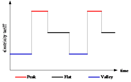
Table 1 lists the main symbols and their definitions in this paper. A typical MDS consists of a water sump to store the mineral water, and several pumps to drain the water from the sump when the water level surpasses the pre-set threshold. Because the electricity consumption varies from period to period in one day, the power supply usually adopts the time-of-use (TOU) electricity tariff mechanism to minimize the pressure on the grid. As shown in Figure 1, the TOU electricity tariff divides one day (24 hours) into several periods, and the electricity tariff in each period may falls into the valley, flat or peak segment. In this case, the pump scheduling is to determine the pump running period that minimizes the electricity consumption and control the water level in the sump under the pre-set threshold.
Table 1. Symbols and definitions
|
Symbol |
Definition |
|
Ht |
Water level at time t |
|
$\phi$ |
The predefined threshold of water level |
|
K |
Number of pumps of an MDS |
|
p |
Power of a pump |
|
L |
Length of predefined time period (unit: minute) |
|
N |
Number of time periods in 24 hours, L·N=1440 minutes |
|
C |
Cost of pumps in 1 day |
|
cp, cf, cv |
Electricity tariff in peak, flat, and valley segment, respectively |
|
ns |
Number of running pumps in sth period, 0≤s≤N |
|
cs |
Electricity tariff in sth period |
|
Hs |
Water level at the beginning of sth period |
|
Fs |
Increased water level by water inflow in sth period |
|
Ds |
Decreased water level by draining water with pumps in sth period |
|
Fs(1) |
Basic exponential smoothing value of Fs |
|
Fs(2) |
Double exponential smoothing value of Fs |
|
$\widehat{H}_{s}$ |
Predicted value of Hs |
|
d |
Decreased water level by one pump in one time period |
|
$\omega$ |
Smoothing factor to compute Fs(1) and Fs(2) |
|
G=(V,E,W) |
Multistage directed and weighted graph for pump schedule |
|
$v_{j}^{(s)} \in \mathrm{V}$ |
A vertex of G, which is in sth stage |
|
$v_{s}^{(0)}, v_{e}^{(N+1)} \in \mathrm{V}$ |
Additional first and last vertex of G |
|
Vs |
Set of vertices of sth stage |
|
wi,j |
Weight of edge $\left\langle v_{i}^{(s)}, v_{j}^{(s+1)}\right\rangle$ |
|
M |
Number of ants of ACO |
|
$\tau_{i, j}$ |
Pheromone laying on edge $\left\langle v_{i}^{(s)}, v_{j}^{(s+1)}\right\rangle$ |
|
$\eta_{i, j}$ |
Locally available heuristic information of edge $\left\langle v_{i}^{(s)}, v_{j}^{(s+1)}\right\rangle$ |
|
$\rho_{i, j}^{A}$ |
Probability of ant A at $v_{i}^{(s)}$ to choose $v_{j}^{(s+1)}$ to visit |
|
$C_{b e s t}$ |
Cost of the best pump schedule |
|
$\alpha, \beta, \rho$ |
Parameters used in ACO |
|
ItrMax |
Maximum number of iterations of ACO |
Figure 1. The TOU electricity tariff
Let Ht be the water level of the sump at time t, ∅ be the pre-set threshold of water level, and K be the number of pumps of an MDS. Meanwhile, it is assumed that the pumps have the same, nonadjustable power p, each day (24 hours) encompasses N periods of equal length L and the same electricity tariff, and the electricity tariffs in peak, flat, and valley segments are cp, cf and cv, respectively. Then, the daily pump cost of the MDS can be expressed as:
$\mathcal{C}=\sum_{i=1}^{K} \int_{0}^{24}(p \cdot r(t) \cdot c(t)) d t$ (1)
where r(t)=0 if the pump is off at time t, and r(t)=1 if the pump is on at time t; c(t) is the electricity tariff at time t. Since each day is divided into several periods, equation (1) can be transformed into:
$\mathcal{C}=\sum_{s=1}^{N} p \cdot n_{s} \cdot c_{s} \cdot L$ (2)
where ns and cs are the number of running pumps and electricity tariff in period s, respectively. Therefore, the pump scheduling problem can be defined as:
$\min \mathcal{C}=\sum_{s=1}^{N} p \cdot n_{s} \cdot c_{s} \cdot L \cdot s \cdot t$
$0 \leq n_{s} \leq K, c_{s} \in\left\{c_{p}, c_{f}, c_{v}\right\}, 0 \leq H_{t} \leq \phi$ (3)
If the water level of the sump is predictable, then the problem defined in equation (3) is to find the ns at the beginning of each period, such that the solution space contains (K+1)N feasible solutions. This task is hard to solve by brute force. This paper adopts the ACO to complete the task. The ACO provides a desirable way to solve discrete optimization problems [15]. This algorithm is inspired by the behavior of real ant colonies: when an ant colony wants to find the shortest path between their nest and a food source, the ants constantly release pheromones, directing each other to resources, while exploring their environment. Each ant constructs a feasible solution and updates the pheromones according to the quality of solution, and the pheromones guide the ants to construct a better solution in the next loop.
4.1 Water level prediction
As mentioned before, each day can be divided into several periods of equal length; in each period, each pump is either in the on state or the off state. Hence, it is necessary to determine the water level at the beginning of each period. Let Hs be the water level at the beginning of period s. Then, the water level at the subsequent period can be calculated as:
Hs+1=Hs+Fs-Ds (4)
where Fs is the water level increase induced by the water inflow; Ds is the water level decrease induced by the water drainage. The value of Ds is already known, as the pump parameters are given in advance. The pumps should be turned on if Hs+1 is greater than the pre-set threshold on water level $\phi$. Since the Fs is constantly changing, the double exponential smoothing was introduced to predict its value.
Let $\omega$ be the smoothing factor. Then, the basic exponential smoothing value of the Fs can be described as:
$\mathrm{F}_{\mathrm{s}+1}^{(1)}=\omega \mathrm{F}_{\mathrm{s}}+(1-\omega) \mathrm{F}_{\mathrm{s}}^{(1)}$ (5)
The double exponential smoothing value of the Fs can be described as:
$\mathrm{F}_{\mathrm{s}+1}^{(2)}=\omega \mathrm{F}_{\mathrm{s}+1}^{(1)}+(1-\omega) \mathrm{F}_{\mathrm{s}}^{(2)}$ (6)
Then, the predicted value of Fs+j can be obtained as:
$\widehat{F}_{s+j}=a_{s}+b_{s} j$ (7)
where
$\left\{\begin{array}{c}{a_{s}=2 F_{s}^{(1)}-F_{s}^{(2)}} \\ {b_{s}=\frac{\omega}{1-\omega}\left(F_{s}^{(1)}-F_{s}^{(2)}\right)}\end{array}\right.$ (8)
The value of Ds depends on the number of running pumps ns and the water level reduction d caused by one pump in each period:
$D_{s}=n_{s} d$ (9)
Therefore, the predicted value of $\widehat{H}_{S+1}$ can be written as:
$\widehat{\mathrm{H}}_{\mathrm{s}+1}=\mathrm{H}_{\mathrm{s}}+\hat{\mathrm{F}}_{\mathrm{s}}-\mathrm{n}_{\mathrm{s}} \mathrm{d}$ (10)
4.2 ACO-based pump scheduling
Before solving the pump scheduling problem by the ACO, the problem defined in equation (3) must be transformed into the shortest path problem in a graph.
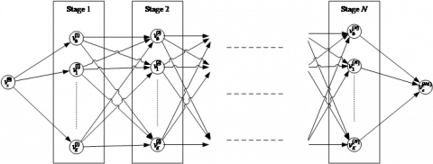
As shown in Figure 2, the pump scheduling problem can be transformed into a multi-stage directed and weighted graph $\mathrm{G}=(\mathrm{V}, \mathrm{E}, \mathrm{W})$, where $\mathrm{V}=\left\{v_{j}^{(s)} | s=1,2, \cdots, N ; j=0,1, \cdots, K .\right\} \cup\left\{v_{s}^{(0)}, v_{e}^{(N+1)}\right\}$, $\mathrm{E}=\left\{\left\langle v_{i}^{(s)}, v_{j}^{(s+1)}\right\rangle\right\} \cup\left\{\left\langle v_{s}^{(0)}, v_{i}^{(1)}\right\rangle\right\} \cup\left\{\left\langle v_{i}^{(N)}, v_{e}^{(N+1)}\right\rangle\right\}$ and $\mathrm{W} : \mathrm{E} \rightarrow \mathbb{R}$ is the weight of edges ( $\mathbb{R}$ is the set of real numbers).
Each period corresponds to one stage in G, and each stage has K vertices corresponding to the K pumps. Let $V_{s}(i=1,2, \cdots, N)$ be the set of vertices in stage s. Then, $\mathrm{V}_{s}=\left\{v_{i}^{(s)} | i=0,1, \cdots, K\right\}$. The weight of $\left\langle v_{i}^{(s)}, v_{j}^{(s+1)}\right\rangle$, wi,j, is the cost incurred by turning on j pumps and turning off i pumps, with $w_{s, i}=w_{i, e}=0(i=1,2, \cdots, K)$. Therefore, the pump scheduling problem is equivalent to finding the shortest path from $v_{s}^{(0)}$ to $v_{e}^{(N+1)}$, which can be solved by the ACO.
Figure 2. The graph of the pump scheduling problem
The basic procedure of the ACO-based pump scheduling plan is as follows:
Step 1: Solution construction. Initially, M ants are all placed at $v_{s}^{(0)}$. In each iteration, each ant chooses the next vertex at a certain probability. For ant A at vertex $v_{i}^{(s)}$, the probability of the ant to visit $v_{j}^{(s+1)}$ can be expressed as:
$\rho_{\mathrm{i}, \mathrm{j}}^{\mathrm{A}}=\frac{\tau_{\mathrm{i}, \mathrm{j}}^{\alpha} \eta_{\mathrm{i}, \mathrm{j}}^{\beta}}{\sum_{\mathrm{j}=0}^{\mathrm{K}} \tau_{\mathrm{i}, \mathrm{j}}^{\alpha} \eta_{\mathrm{i}, \mathrm{j}}^{\beta}}$ (11)
where $\tau_{i, j}$ and $\eta_{i, j}=\frac{1}{w_{i, j}}$ are the pheromone and local heuristic information of $\left\langle v_{i}^{(s)}, v_{j}^{(s+1)}\right\rangle$, respectively; $\alpha$ and $\beta$ are the relative importance parameters of $\tau_{i, j}$ and $\eta_{i, j}$, respectively. If several vertices have the same probability, the ant will select one of them by random.
In addition, the solution construction of each ant must satisfy the constraints in equation (3). The first constraint, $0 \leq n_{s} \leq K$, is automatically satisfied, because $0 \leq\left|\mathrm{V}_{s}\right| \leq K$; the second constraint, $c_{s} \in\left\{c_{p}, c_{f}, c_{v}\right\}$, is used to compute the cost of each solution; the third constraint, $0 \leq H_{t} \leq \phi$, is satisfied if the next vertex is not $v_{0}^{(s+1)}$ if ant A is at vertex $v_{i}^{(s)}$, and $\widehat{H}_{s+1}>\phi$ or $\widehat{H}_{s+2}>\phi$.
Step 3: Pheromone update. After all ants have constructed their solutions, the pheromone trails are updated by the following rule:
$\tau_{i, j}=(1-\rho) \tau_{i, j}+\Delta \tau_{i, j}^{b e s t}$ (12)
where $0<\rho \leq 1$ is the pheromone evaporation rate; $\Delta \tau_{i, j}^{b e s t}$ is the amount of pheromone released by the ants on $\left\langle v_{i}^{(s)}, v_{j}^{(s+1)}\right\rangle$, which can be defined as
$\Delta \tau_{i, j}^{b e s t}=\left\{\begin{array}{cc}{\frac{1}{C_{b e s t}}} & {\text { if }\left\langle v_{i}^{(s)}, v_{j}^{(s+1)}\right\rangle \text { is in the best solution }} \\ { 0} & {\text { otherwise }}\end{array}\right.$ (13)
Based on the above description, the ACO-based pump scheduling algorithm was summed up as follows:
Algorithm 1. CEPS algorithm
|
|
Function CEPS (G)// G is the graph as Figure 2 |
|
|
Set parameters and initialize pheromone trails; |
|
|
for Itr $\leftarrow 1$ to ItrMax |
|
|
for $i \leftarrow 1$ to M |
|
|
List $_{0}^{\mathrm{i}} \leftarrow \mathrm{v}_{\mathrm{s}}^{(0)}$ |
|
|
for $j \leftarrow 1$ to N+1 |
|
|
$\mathbf{u} \leftarrow$ List $_{j-1}^{\mathrm{i}}$ |
|
|
$\mathrm{v} \leftarrow \operatorname{argmax}\left\{\rho_{\mathrm{u}, \mathrm{v}}^{\mathrm{i}} | \rho_{\mathrm{u}, \mathrm{v}}^{\mathrm{i}} \text { computed by }(11) \text { and v satisfying constraints of $(3)$}\right\}$ |
|
|
List $_{\mathrm{j}}^{\mathrm{i}} \leftarrow \mathrm{v}$ |
|
|
end for |
|
|
end for |
|
|
List$_{\text { best }}^{\text { Itr }}$ $\leftarrow$ shortest path of this iteration |
|
|
$C_{\mathrm{best}}^{\mathrm{Itr}} \leftarrow \operatorname{cost}$ of List $_{\mathrm{best}}^{\mathrm{Itr}}$ |
|
|
List$_{\text { best }}^{\text { global }}$ $\leftarrow$ shortest path so far |
|
|
$\mathcal{C}_{\text { best }}^{\text { global }} \leftarrow$ cost of List$_{\text { best }}^{\text { global }}$ |
|
|
update $\tau$ according to (12) and (13) |
|
|
end for |
|
|
return List$_{\text { best }}^{\text { global }}$ and $\mathcal{C}_{\text { best }}^{\text { global }}$ |
|
|
end function |
From September 1st to 30th, 2018, several experiments were carried out on the real data of Jinchiling Gold mine in Zhaoyuan, eastern China’s Shandong Province, to verify the feasibility of the proposed algorithm. One MDS with K=5 pumps was selected for the experiments from the mine. The power of each pump is p=110 kW. The water level threshold of the sump is $\phi=2.2 \mathrm{m}$. The TOU electricity tariff is given in Table 2, where cp , cf and cv are respectively RMB 1.252-yuan, 0.782 yuan and 0.370 yuan. Each day (24h) was divided evenly into N=72 periods with the length L=20 minutes. The smoothing factor was set to $\omega=0.7$. The symbols and their definitions were given in Table 3 below.
Table 2. TOU electricity tariff
|
Time period |
0:00-6:00 |
6:00-8:00 |
8:00-11:00 |
11:00-18:00 |
18:00-21:00 |
21:00-24:00 |
|
Tariff (Unit: Yuan) |
0.370 |
0.782 |
1.252 |
0.782 |
1.252 |
0.370 |
Table 3. Symbols and definitions
|
Period |
1 |
2 |
3 |
4 |
5 |
6 |
7 |
8 |
9 |
|
Fs |
2.095 |
2.107 |
2.118 |
2.126 |
2.135 |
2.147 |
2.158 |
2.169 |
2.180 |
|
$\hat{F}_{s+1}$ |
2.095 |
2.112 |
2.126 |
2.135 |
2.144 |
2.158 |
2.169 |
2.180 |
|
|
$\hat{F}_{s+2}$ |
2.095 |
2.118 |
2.135 |
2.143 |
2.153 |
2.168 |
2.180 |
||
|
$\hat{F}_{s+3}$ |
2.095 |
2.124 |
2.144 |
2.152 |
2.162 |
2.179 |
|||
|
Period |
10 |
11 |
12 |
13 |
14 |
15 |
16 |
17 |
18 |
|
Fs |
2.188 |
2.200 |
2.209 |
2.220 |
2.221 |
2.221 |
2.302 |
2.310 |
2.322 |
|
$\hat{F}_{s+1}$ |
2.190 |
2.197 |
2.210 |
2.220 |
2.230 |
2.228 |
2.225 |
2.336 |
2.341 |
|
$\hat{F}_{s+2}$ |
2.191 |
2.201 |
2.207 |
2.221 |
2.230 |
2.241 |
2.234 |
2.227 |
2.376 |
|
$\hat{F}_{s+3}$ |
2.191 |
2.201 |
2.212 |
2.216 |
2.232 |
2.240 |
2.251 |
2.240 |
2.230 |
|
Period |
19 |
20 |
21 |
22 |
23 |
24 |
25 |
26 |
27 |
|
Fs |
2.329 |
2.337 |
2.348 |
2.356 |
2.364 |
2.373 |
2.382 |
2.391 |
2.403 |
|
$\hat{F}_{s+1}$ |
2.343 |
2.343 |
2.347 |
2.358 |
2.365 |
2.373 |
2.382 |
2.390 |
2.400 |
|
$\hat{F}_{s+2}$ |
2.369 |
2.362 |
2.355 |
2.357 |
2.368 |
2.374 |
2.381 |
2.391 |
2.399 |
|
$\hat{F}_{s+3}$ |
2.417 |
2.397 |
2.381 |
2.367 |
2.366 |
2.378 |
2.383 |
2.390 |
2.400 |
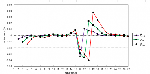
Figure 3. Relative errors of predicted values
Figure 3 records the relative errors of the predicted values of 27 water inflow levels (Fs) in one day. It can be seen that $\hat{F}_{s+1}$ is the most accurate. The mean relative errors of $\hat{F}_{s+1}$, $\hat{F}_{s+2}$ and $\hat{F}_{s+3}$ are, respectively, 0.039 %, 0.066 %, and 0.091 %. The water level variation at 16 causes the greatest prediction error.
Using the above prediction data, the pump scheduling was carried out by Algorithm 1. For convenience, the original pump scheduling plan is denoted as the original plan, and the pump scheduling plan after the optimization by Algorithm 1 is denoted as the optimized plan. Note that the latter plan is simulated rather than the real scheduling of Jinchiling gold mine.
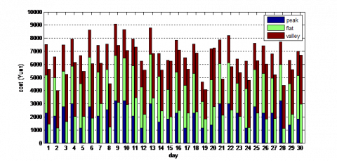
The ACO parameters were directly extracted from Reference [16], which also finds the shortest path in a graph by the ACO, including M = 30 ants, $\alpha=1$, $\beta=2$, $\rho=0.9$ and $\operatorname{ItrMax}=300$. The costs of original and optimized plans are compared in Table 4 and Figure 4. The comparison shows that Algorithm 1 can reduce the mine operation cost by 34.09 % on average from the level of the original plan.
Table 4. Total costs of the original and optimized plans (Unit: RMB yuan)
|
Day |
1 |
2 |
3 |
4 |
5 |
6 |
7 |
8 |
9 |
10 |
|
Original |
7507 |
6562 |
7474 |
7931 |
6678 |
8611 |
7461 |
7553 |
9084 |
8641 |
|
Optimized |
4230 |
3671 |
4696 |
5547 |
5079 |
4781 |
5165 |
5369 |
6389 |
6559 |
|
Day |
11 |
12 |
13 |
14 |
15 |
16 |
17 |
18 |
19 |
20 |
|
Original |
7932 |
6254 |
8785 |
6823 |
6307 |
7835 |
6502 |
7533 |
4655 |
7198 |
|
Optimized |
5274 |
4702 |
5458 |
5413 |
4127 |
6061 |
3456 |
3850 |
3560 |
4015 |
|
Day |
21 |
22 |
23 |
24 |
25 |
26 |
27 |
28 |
29 |
30 |
|
Original |
7888 |
8190 |
6426 |
6246 |
7608 |
7423 |
6813 |
7721 |
6304 |
7010 |
|
Optimized |
5151 |
4661 |
3480 |
4019 |
4562 |
5666 |
4274 |
5362 |
4504 |
4981 |
Figure 4. Cost comparison between the original and optimized plans
(In each pair of bars, the left and right bars are respectively the costs of the original and optimized plans.)
Table 5 shows the machine hours of the pumps in peak, flat and valley periods of the two plans. It can be seen that the optimized plan greatly reduces the machine-hours in peak period, and increases the machine-hours in valley period. The results are consistent with Figure 4, where the cost in peak period only accounts for a fraction of the total cost.
Table 5. Machine-hours of the pumps in the original and optimized plans in different periods
|
Time period |
Peak |
Flat |
Valley |
|
Original |
17.67 |
39.21 |
54.62 |
|
Optimized |
2.65 |
27.99 |
98.55 |
With pumps as the main devices, the MDSs often consume lots of electricity in mine production. In most mines, the TOU electricity tariff mechanism is adopted because the pumps only start when the water level in the sump reaches a pre-set threshold. Thus, pump scheduling is a possible way to optimize the MDS energy efficiency. This paper utilizes double exponential smoothing method to predict the water inflow, and employs the ACO to obtain the optimal pump scheduling plan. The proposed pump scheduling method was verified through experiments in a gold mine in China. The experimental results show that the optimized plan can greatly reduce the mine operation cost. The future research will explore the pump scheduling of MDSs with different types of pumps.
This paper is made possible thanks to the National Key Research and Development Plan of China (Grant No.: 2018YFC1406203; 2017YFC0804406)
[1] Zhang, Z., Meng, G., Wang, A. (2018). Numerical simulation of scale removal from mine drainage pipe by water jet. Journal of Applied Science and Engineering, 21(2): 145-154. https://doi.org/10.6180/jase.201806_21(2).0001
[2] Han, C.H., Xue, S.X., Cao, S.L., Chen, Z.W. (2017). Experimental research for system energy conservation of the drainage pumping station. Fluid Mach, 45(2): 1-5. https://doi.org/10.3969/j.issn.1005-0329.2017.02.001
[3] Liu, W., Zhou, S., Li, C. (2018). Operation of mine pump units based on artificial bee colony algorithm. Fluid Mach, 46(1): 56-61. https://doi.org/10.3969/j.issn.1005-0329.2018.01.012
[4] Wei, X., Zhang, S., Han, Y., Wolfe, F.A. (2017). Mine drainage: Research and development. Water Environ. Resour, 89(10): 1384-1402. https://doi.org/10.2175/106143017X15023776270377
[5] Vieira, T.P., Almeida, P.E.M., Meireles, M.R.G. (2018). Use of computational intelligence for scheduling of pumps in water distribution systems: A comparison between optimization algorithms, in Proc. IEEE Congr. Evol. Comput., 8-13 July, Rio de Janeiro, Brazil, IEEE: New York, USA, pp. 1-8. https://doi.org/10.1109/CEC.2018.8477833
[6] Fooladivanda, D., Taylor, J.A. (2018). Energy-optimal pump scheduling and water flow. IEEE Trans. Control Netw. Syst, 5(3): 1016-1026. https://doi.org/10.1109/TCNS.2017.2670501
[7] Chazarra, M., Pérez-Díaz, J.I. (2018). García-González, J. Optimal joint energy and secondary regulation reserve hourly scheduling of variable speed pumped storage hydropower plants. IEEE Trans. Power Syst, 33(1): 103-115. https://doi.org/10.1109/TPWRS.2017.2699920
[8] Zhang, L., Zhuan, X. (2017). Optimal operation scheduling of multiple pump units on variable speed operation with VFD in the east route of south-to-north water diversion project. in Procs. 36th Chinese Control Conf., 26-28 July, Dalian, China, IEEE: New York, USA, pp. 2818-2823. https://doi.org/10.23919/ChiCC.2017.8027792
[9] Soonthornnapha, T. (2017). Optimal scheduling of variable speed pumps in Mahasawat water distribution pumping station, in Procs. Inter. Electr. Engin. Congr. 8-10 March, Pattaya, Thailand, IEEE: New York, USA, pp. 1-4. https://doi.org/10.1109/IEECON.2017.8075752
[10] Gao, Z.Z., Zhao, C.H., Shang, C.L., Tan, C. (2017). The optimal control of mine drainage systems based on hybrid Petri nets, in Procs. Chinese Autom. Congr. 20-22 Oct., Jinan, China, IEEE: New York, USA, pp. 78-83. https://doi.org/10.1109/CAC.2017.8242740
[11] Dong, D., Sun, W., Xi, S. (2012). Optimization of mine drainage capacity using FEFLOW for the No. 14 coal seam of China’s Linnancang coal mine. Mine Water Environ, 31: 353-360. https://doi.org/10.1007/s10230-012-0205-5
[12] Li, C.L., Fan, J.C., Peng, Y., Lian, J., Zhou, S.P. (2016). Optimal operation of mine pump units based on genetic algorithms. J. East China Univ. Sci. Techn. (Nat. Sci. Ed.). 42(2): 266-270. https://doi.org/10.14135/j.cnki.1006-3080.2016.02.018
[13] Ren, Z., Han, J. (2015). Energy saving control research on mine drainage system based on model predictive control. J. Syst. Simul, 27(12): 3032-3037. https://doi.org/10.16182/j.cnki.joss.2015.12.022
[14] Hou, J. (2014). Research on dynamic gray forecast for mine inflow and drainage energy control. Comput. Syst. Appl, 23(3): 203-207. https://doi.org/10.3969/j.issn.1003-3254.2014.03.038
[15] Dorigo, M., Stützle, T. (2013). Ant colony optimization: Overview and recent advances. in Handbook of metaheuristics. M. Gendreau and J.-Y. Potvin, Eds, 146: 311-351. https://doi.org/10.1007/978-1-4419-1665-5_8
[16] Wang, Y.L., Cui, H.Q., Guo, Q., Shu, M.L. (2013). Obstacle-avoidance path planning of a mobile beacon for localization. IET Wireless Sensor Syst, 3(2): 126-137. https://doi.org/10.1049/iet-wss.2011.0128