Bayu Adhi Prakosa*![]() | Yuggo Afrianto
| Yuggo Afrianto![]() | Seno Agustiyan
| Seno Agustiyan![]() | Ibnu Hanafi Setiadi
| Ibnu Hanafi Setiadi
© 2024 The authors. This article is published by IIETA and is licensed under the CC BY 4.0 license (http://creativecommons.org/licenses/by/4.0/).
OPEN ACCESS
For computer networks, bandwidth management is essential. Bandwidth management is a strategy used in network administration to try and provide fair and acceptable network performance. Researchers have monitored the effectiveness of bandwidth management methods including Per Connection Queue (PCQ), Random Early Detection (RED), and First In First Out (FIFO) schemes using the Simple Network Management Protocol (SNMP) protocol. (1) To ascertain which of the PCQ, RED, and FIFO bandwidth management techniques performs best is the main goal of this study. (2) Is able to forecast how well bandwidth management techniques will function on a network, providing a guide for putting the best techniques into practice. This study included a variety of methodologies, including testing, design, implementation, and analysis. The PCQ method performs better than the RED or FIFO methods when monitored using the SNMP protocol and the Cacti application as an interface. Predictions using multiple linear regression on bandwidth management methods are used to estimate the CPU and memory performance of the PCQ, RED, and FIFO Mikrotik routers that are implemented on the network constructed by researchers. Compared to the prediction accuracy on CPU performance, which has a total average error value of 0.9204, the memory performance prediction accuracy using multiple linear regression is more accurate, with a total average error value of 0.0315.
bandwidth management, Per Connection Queue (PCQ), Random Early Detection (RED), First In First Out (FIFO), prediction, linear regression, Simple Network Management Protocol (SNMP), cacti, Mikrotik
The control of bandwidth is crucial for computer networks. One method of network management used to try to achieve equitable and acceptable network performance is bandwidth management [1]. Broadband use is frequently not used to its full potential. One or more customers that utilize bandwidth capacity for downloading or accessing programs that use bandwidth capacity may be the source of this [2].
Naturally, while adopting bandwidth management, it must take into account the requirements set out by a network [3]. poor network performance and poor resource utilization result from either overuse or underuse of the network's bandwidth, which leads to subpar network performance [4]. As a result, it becomes crucial to make sure that a network's capacity matches the amount of accessible bandwidth [5]. Naturally, the router is a key component in bandwidth management operations [6]. One network device with dependable qualities is a proxy router [7]. Naturally, using the network has an impact on the router's performance, which in turn has an impact on how well a network is optimized [8]. To gain best network performance, of course, there are numerous queuing methods that may be utilized as bandwidth management methods. These queuing methods contain algorithms for running queues of data packets in and out of a network [9].
The PCQ approach, which enables the equitable distribution of bandwidth limits on a network, is one of the queuing techniques used for bandwidth control. Because the use of queues will be complex, this strategy is frequently employed on networks with a high number of clients or on networks where it is difficult to anticipate the number of customers [10]. Next is the Random Early Detection, or RED, approach. Through the use of random marking or dropping, this technique can remove data packets from a network before congestion arises [11]. Additionally, the simplest way—which is typically the default method that is active on network devices—is the FIFO (First In, First Out) approach. Incoming data packets are briefly held in a basic buffer using this approach, and there is no priority given to the incoming data [12]. Numerous studies have examined bandwidth management techniques prior to use multiple linear regression to estimate the performance of PCQ, RED, and FIFO systems. This includes studies conducted by Iswadi et al. [13] that has analyzed network bandwidth management at Siliwangi University by recommending the PCQ method, where the research uses the PCQ method as a queue type or queuing method. Research from Tilaye and Gojeh [14] has conducted research on Comparison of Bandwidth Management Using the FIFO (First-In, First-Out) and PCQ (Per Connection Queue) Methods on Mikrotik Routers (Case Study of Network Computer Laboratory, AKPRIND Institute of Science and Technology Yogyakarta) where in this study, namely comparing QOS (quality of service) FIFO and PCQ methods with a proxy router as a network device that implements the FIFO and PCQ methods. Nurfiana has conducted research on the implementation of the PCQ-Queue Tree Method on Mikrotik Routers and Cacti Monitoring for Quality of Service Improvement where, in the utilization of the PCQ-queue tree method, network traffic monitoring is also carried out on proxy routers using the Cacti application, which can monitor in real time to improve the quality of service on the network [15]. Adams 's [16] research has conducted Research on Analysis and Implementation of the Random Early Detection (RED) Method on TCP and IP Networks, which in this study uses the RED queuing method for bandwidth management utilization in TCP and IP networks. Research from Sapalo Sicato et al. [17] on the Implementation of Simple Queue and Website Filter for Bandwidth Management Optimization at the Mediterranean Apartment, where this research uses simple queue and website filters to optimize bandwidth management and uses the FIFO method as a queuing method for bandwidth management. Research from Lipsky and Church [18] on the PCQ and Queue Tree Methods for the Implementation of Mikrotik-Based Bandwidth Management aims to facilitate bandwidth management with limited existing bandwidth using the PCQ method. Research from Nendi and Dennis Andika Putra on Bandwidth Management with Peer Connection Queue (PCQ) and Simple Queue Methods in PPH 2 Housing which this research implements the PCQ method through a simple queue in PPH 2 housing so that it can facilitate bandwidth management with limited existing bandwidth and make maximum use of internet connections [19]. Research from Muhammad Rafi and his colleagues on Comparative Analysis of Bandwidth Management with Random Early Detection (RED) and Class-Based Queue (CBQ) Methods at Telkom University Landmark Tower (TULT) which in this study compares bandwidth management, namely RED and CBQ methods, with quality of service parameters [20]. Research from Azriel Christian Nurcahyo and his colleagues on Comparison of RED, SFQ, and AQM Algorithms on Enterprise Networks with Vmware Esxi and Router OS where this research compares the RED, SFQ, and AQM algorithms performed on OS routers integrated with Vmware ESXI [21]. Research from Mochammad Arya Darmawan and his colleagues on Bandwidth Management on Mikrotik with Multilevel Limitation Using the Simple Queue Method which this research does bandwidth limitation using the simple queue method with multilevel limitation, where the implementation uses queue parent and child parent, Queue parent is the total bandwidth owned, and child parent is the bandwidth limit set on the client based on the IP address [22].
There are similarities and differences between this study and the ten earlier studies. The PCQ, RED, and FIFO methods are used in both studies to manage bandwidth on Mikrotik routers. However, this study uses multiple linear regression to predict how well the PCQ, RED, and FIFO methods will perform in terms of the CPU and memory usage of the proxy router. Multiple linear regression offers advancements that can improve network performance analysis and forecasting when applied to bandwidth management, particularly when contrasting bandwidth-management techniques. Multiple linear regression allows for the modeling of complex relationships between input variables (like traffic values for ping latency, inbound, and outbound traffic) and output variables (like CPU and memory usage on the router). The relative impact of each variable on the router's resource consumption can thus be determined.
In this study, the issue is that networks frequently experience subpar network performance, because of network conditions that frequently exhibit fluctuations in user numbers and application types, and obstacles that develop in the functioning of network devices, especially routers, which have an effect on network optimization [23]. Because Mikrotik routers have multiple bandwidth management techniques, including PCQ, RED, and FIFO, an optimal bandwidth management method is therefore required. The actions made to manage the network are ineffective since the effects of these changes on network performance are frequently unpredictable.
Finding the performance outcomes of bandwidth management techniques on a network, namely PCQ, RED, and FIFO, as well as the methods' performance forecast accuracy, are the main objectives of this study.
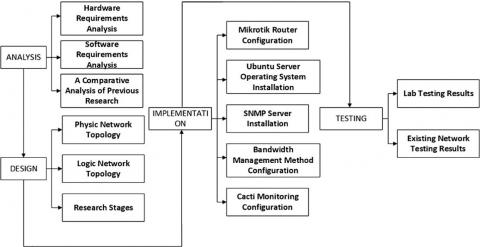
This research methodology can be considered a structured framework for organizing concepts or a system for executing actions that are focused and relevant to the goals and objectives of the study (Figure 1).
Figure 1. Research methods
2.1 Analysis
The analysis phase, which is the process of evaluating and figuring out what is required in the research to be conducted, starts the first phase [24].
2.1.1 Hardware requirement analysis
At this point, the hardware or hardware requirements needed for research are being prepared.
2.1.2 Software requirements analysis
Following the completion of the hardware requirements analysis stage, the software requirements are prepared in order to conduct this research at the software requirements analysis stage.
2.1.3 A comparative analysis of previous research
This stage involves a comparative analysis of the benefits and drawbacks of the PCQ, RED, and FIFO methods from earlier studies.
2.2 Design
The design step involves creating a model or simulation of the system or network architecture that will be implemented. It's also anticipated that this description would give a thorough picture of the requirements as they stand, whether they take the shape of a study's system architecture or network topology [25].
2.2.1 Physic topology design
Creating a diagram or topology design that depicts the network devices that are connected to one another is known as the physical topology design step.
2.2.2 Logic topology design
Subsequently, at the step of logic topology design, a topology description or design explaining the IP address addressing on the network used for the study is created.
2.2.3 Research stages
And at the research stage, which delineates the steps taken from the start of the research process to the acquisition of research findings.
2.3 Implementation
Implementation refers to carrying out all of the plans made during the requirements analysis and design phases of the preceding process. And at this point, the implementation phase is what decides if the planned study will be successful or unsuccessful [26].
2.3.1 Mikrotik router configuration
Setting up a proxy router to allow the researchers' network to be linked and utilized for PCQ, RED, and FIFO research technique comparisons.
2.3.2 Ubuntu server operating system installation
The Ubuntu server operating system is installed and will be used as the operating system for the server machine that will keep track of how well the proxy router's bandwidth control technique is working.
2.3.3 SNMP server installation
Subsequent to the installation of the Ubuntu server operating system on the server computer, the SNMP protocol will be installed on the operational server computer. The purpose of this protocol is to monitor real-time data pertaining to the proxy router's functioning.
2.3.4 Bandwidth management method configuration
Configure the PCQ, RED, and FIFO bandwidth control techniques on the proxy router once all necessary hardware and software have been installed and operating.
2.3.5 Cacti monitoring configuration
Next, some real-time data graphs of proxy router performance are added to the Cacti program, which serves as an interface for tracking the effectiveness of the bandwidth control technique.
2.4 Testing
The term "testing stage" describes a set of methods and approaches used to put the research's hypothesis or theory to the test. In order to validate or invalidate the theory or hypothesis being investigated, this test aims to generate empirical data [27].
2.4.1 Lab testing results
The PCQ, RED, and FIFO methods of bandwidth management on Mikrotik routers, as well as predictions about their performance, were the focus of this lab test, which was conducted on the network of the Computer System and Network laboratory of Ibn Khaldun University Bogor.
2.4.2 Existing network testing results
Additionally, just like with the lab test, the existing network test is conducted solely in the center of the Ibn Khaldun University Bogor Rectorate Building.
The findings of the four steps of the study, first analysis, second design, third implementation, and fourth testing, were used to predict the performance of the PCQ, RED, and FIFO methods using multiple linear regression on SNMP-based Mikrotik routers.
3.1 Analysis
It may be inferred from the issues and plans raised during the analysis stage that a number of requirements must be satisfied prior to carrying out this study, including:
3.1.1 Hardware requirements analysis
The required gadgets for this research are listed in Table 1.
Table 1. Hardware requirements analysis
|
No. |
Hardware |
Total |
Specifications |
Function |
|
1 |
Router Mikrotik |
2 |
RB751U-2HnD, CPU AR7241 400 MHz, RAM: 32 MB, HDD: 64 MB. RB1100Dx4, CPU ARMv7 1.4 GHz, RAM: 1 GB, HDD: 128 MB |
-As an internet connection provider -To implement the bandwidth management method |
|
2 |
Personal Computer |
1 |
-Intel Core i5-7500 CPU 3.40GHz x 4, RAM: 4 GB |
As a monitoring server |
3.1.2 Software requirements analysis
The software prepared to run this research is listed in Table 2.
Table 2. Software requirements analysis
|
No. |
Software |
Function |
|
1 |
Ubuntu Server 20.04.3 |
The operating system used as a Mikrotik router monitoring server |
|
2 |
Cacti |
Software for Mikrotik router CPU monitoring interface |
|
3 |
Winbox |
Software for configuring Mikrotik routers |
|
4 |
Microsoft Excel |
Software to calculate the linear regression prediction formula |
3.1.3 A comparative analysis of previous research
Table 3 presents a comparison of the key findings from the previous ten studies regarding the benefits and drawbacks of the PCQ, RED, and FIFO methods:
Table 3. A comparative analysis of previous research
|
No. |
Methods |
Advantages |
Disadvantages |
|
1 |
PCQ |
- Permits equitable bandwidth sharing between open connections - Ideal for networks with different client counts |
- Performance of PCQ may be impacted by a large increase in the number of connections, requires ongoing observation and modification |
|
2 |
RED |
- Can identify and drop packets before congestions occur, maintaining low latency for users |
- Unwanted packet drop rates may result from incorrect parameter selection in the configuration |
|
3 |
FIFO |
- Ascertain package delivery according to arrival order, according to honest and open standards |
- The requirements of particular applications or service kinds cannot be used to prioritize or arrange delivery |
(1) Network scalability capability
As for networks operating in real time, RED is better suited for preventing congestions, while the PCQ method works well with large numbers of connections or high client fluctuations. In complex networks with varied traffic, FIFO, despite its simplicity, may not be as effective.
(2) Configuration flexibility
PCQ allows for fair bandwidth distributing and priority setting flexibility, but requires careful management to maintain optimal performance. While RED requires careful parameter configuration for its effectiveness, and FIFO, while easy to manage, has limitations in priority setting.
While weighing the benefits and drawbacks of each approach, the right choice for bandwidth management on MikroTik routers must also consider the unique features and goals of the network being managed. Prior studies have yielded insightful findings in this area.
3.2 Design
A network topology design and a summary of the phases of the study, from the start of the investigation to the findings, are among the many designs or pictures that come from the research that was conducted.
3.2.1 Physic topology design
The Physic topology design in this study describes the network devices connected to each other in the CSN lab room as well as a local network linked to the Ibn Khaldun University Bogor Rectorate Building's central network. Ethernet1 connects router RB1100Dx4 (Router Core), also known as the central router in the Rectorate Building of Ibn Khaldun University Bogor, to the internet network. Ethernet5 connects router RB1100Dx4 (Router Core) to the Switch (Rectorate), which is connected to the Faculty of Engineering network and to the CCR1009-7G-1C-1S+ router. Next, using the Cisco SF 100-24 port 10/100 Switch (FT CENTER), which is also connected to the Rise Center Building, the CCR1009-7G-1C-1S+ router is re-deployed on its local interface. Switch 02 is then connected to Switch 03 CSN Lab Room.
3.2.2 Logic topology design
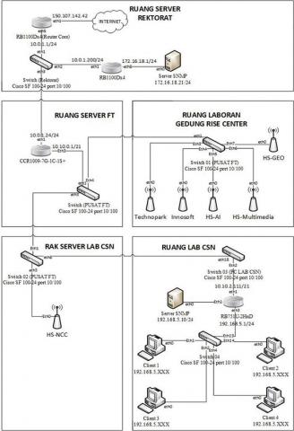
Researchers constructed a network structure in the CSN Lab room, and the local network structure connected to the network center of the Ibn Khaldun University Bogor Rectorate Building, all describe the logic topology that explains the IP Address management of interconnected network devices. IP address 10.0.1.1 is a local IP address connected to the Faculty of Engineering network, and IP address 172.16.18.21 is on the SNMP server in the Rectorate Server room as it monitors the performance of the RB1100Dx4 router (Router Core) connected to the internet, and the Faculty of Engineering network through the CCR1009-7G-1C-1S+ router has an IP address of 10.0.1.24 to connect with the Rectorate Building network, and IP address 10.10.0.1 as a Local IP connected to the Rise Center Building and CSN Lab (Figure 2).
3.2.3 Research stages
The research stages describe the flow of a work process, to predict the performance of the PCQ, RED, and FIFO methods. First, install a computer network such as configuration on the router, namely IP address configuration, DHCP, and NAT (Figure 3). Next, set up the PCQ, RED, and FIFO methods through a proxy router. Researchers in the Computer System and Network Laboratory then tested the network scheme by streaming video from all client computers connected to it. Then, using an SNMP server with a cacti interface, monitor the performance of the bandwidth management methods on the central network of the Ibn Khaldun University Bogor Rectorate Building. The performance of the PCQ, RED, and FIFO methods is then predicted using the multiple linear regression method training. Finally, real data is obtained by repeating the monitoring process and combining it with the outcomes of the multiple linear regression prediction training to obtain PCQ, RED, and FIFO method prediction data. The following is an overview of the stages of research conducted.
Figure 2. Network topology
Figure 3. Research stages
3.3 Implementation
In order for the study to proceed as planned at this point of implementation, the design created in earlier phases must be applied or implemented.
3.3.1 Mikrotik router configuration
Setting up the IP address on the local and internet interfaces is the first step towards enabling the proxy router to function as intended. Next, DHCP Server and Client must be configured to provide automatic IP addresses, and finally, NAT must be configured to enable local networks to connect to public networks.
3.3.2 Ubuntu server operating system installation
The way to do this is to install the Ubuntu Server operating system, specifically on the machine acting as a server (Ubuntu Server 20.04.3 in this case).
3.3.3 SNMP server installation
Ubuntu Server, an operating system designed to perform network-based functions, can be used to install the SNMP protocol at this point in the SNMP server installation process. Install Apache as a web server after installing the SNMP protocol. Then install PHP and MYSQL to install PHP programming and database on the web server. Then install the cacti application as an interface for network monitoring.
3.3.4 Bandwidth management method configuration
Next, set up the proxy router's bandwidth management techniques, which are the PCQ, RED, and FIFO methods used on the basic queue feature with queue type selection for upload and download targets aimed at the aforementioned techniques.
3.3.5 Cacti monitoring configuration
By identifying the networked target devices, you can set up the Cacti application to monitor proxy router devices. You can then add graphs to gather real-time monitoring data on the proxy router's performance.
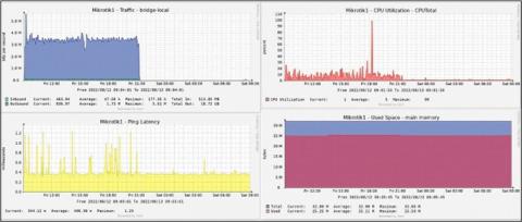
The results of network monitoring that was conducted for a full day, from August 12, 2022, at 9 a.m., to August 13, 2022, at 9 a.m., can be seen after completing the following steps. as seen in the image below.
Figure 4. Traffic volume on the network
Figure 5. Performance monitoring of bandwidth management
Additionally, the monitoring results above show that during working hours, network traffic is extremely high, between 9:00 a.m. and 9:00 p.m., with a 3.5 Mbps average and a 1.81 Mbps total (Figure 4).
3.4 Testing
In addition to the core network of the Ibn Khaldun University Bogor Rectorate Building, which is tested as an existing network during business hours and sees heavy network traffic, tests were conducted on the computer system and network laboratory network.
3.4.1 Performance analysis results of bandwidth management methods
To test the designated network and track the performance of the proxy router in order to obtain the performance results of the bandwidth management method from this study (Figure 5).
(1) Performance monitoring results of PCQ method
When using the PCQ method, the average performance is obtained with the parameters of inbound traffic, outbound traffic, ping latency, CPU utilization, and main memory on the proxy router. The PCQ method is tested to determine its performance based on the results of monitoring on the SNMP server accessed through the Cacti software interface (Table 4).
Table 4. PCQ method performance
|
PCQ Performance |
Average |
|
CPU |
5 (%) |
|
Memory |
25.19 (MB) |
|
Ping Latency |
406.08 (ms) |
|
Traffic Inbound |
3.56 (Mbps) |
|
Traffic Outbound |
3.42 (Mbps) |
(2) RED method performance monitoring results
After testing the RED method using the results of monitoring on the SNMP server accessed through the Cacti software interface, the average performance is obtained when implementing the RED method with the parameters of inbound traffic, outbound traffic, ping latency, CPU utilization, and main memory on the proxy router (Table 5).
Table 5. Performance of RED method
|
RED Performance |
Average |
|
CPU |
9 (%) |
|
Memory |
24.54 (MB) |
|
Ping Latency |
4766.92 (ms) |
|
Traffic Inbound |
5.68 (Mbps) |
|
Traffic Outbound |
5.14 (Mbps) |
(3) FIFO method performance monitoring results
In order to assess the effectiveness of the FIFO method, monitoring data from the SNMP server accessed via the Cacti software interface is used. When applying the FIFO method, the proxy router's main memory, ping latency, inbound and outbound traffic, CPU utilization, and main traffic are used to calculate the average performance (Table 6).
Table 6. FIFO Method Performance
|
FIFO Performance |
Average |
|
CPU |
5 (%) |
|
Memory |
24.39 (MB) |
|
Ping Latency |
3301.36 (ms) |
|
Traffic Inbound |
3.44 (Mbps) |
|
Traffic Outbound |
3.24 (Mbps) |
The performance of the PCQ, RED, and FIFO methods are obtained. Next, a comparison is made by assigning points to each performance value, namely CPU Utilization, Memory, Ping Latency, Inbound Traffic, and Outbound Traffic, where the smallest performance value has the largest percentage point value. This allows for the determination of which method performs at the best level.
$p=100-|| \frac{n}{\sum n}|100|$ (1)
where p is the performance point and n is the average performance value, each performance value of the PCQ, RED, and FIFO methods will be calculated using the percentage formula [28], these calculations and their outcomes are summarized in Table 7.
Table 7. Performance comparison of bandwidth management methods
|
Methods |
Average Performance and Performance Points |
Total Point |
||||
|
CPU Utilization |
Memory |
Ping Latency |
Traffic Inbound |
Traffic Outbound |
||
|
PCQ |
5 |
25.19 |
406.08 |
3.56 |
3.42 |
|
|
PCQ Point |
73.7 |
66 |
95.2 |
71.9 |
71 |
377.8 |
|
RED |
9 |
24.54 |
4766.92 |
5.68 |
5.14 |
|
|
RED Point |
52.6 |
66.9 |
43.7 |
55.2 |
56.4 |
274.9 |
|
FIFO |
5 |
24.39 |
3301.36 |
3.44 |
3.24 |
|
|
FIFO Point |
73.7 |
67.1 |
61 |
72.9 |
72.5 |
347.2 |
Table 8. Bandwidth management method performance sample data
|
No. |
Date |
Traffic Inbound (MBPS) |
Traffic Outbound (MBPS) |
Ping Latency (MS) |
CPU Utilization (%) |
Main Memory (MB) |
|
1 |
8/11/2022 9:10 |
0.05 |
0.1 |
343.08 |
4 |
25.26 |
|
2 |
8/11/2022 9:15 |
1.37 |
1.34 |
590.34 |
17 |
25.26 |
|
3 |
8/11/2022 9:20 |
3.33 |
3.15 |
592 |
16 |
25.56 |
|
4 |
8/11/2022 9:25 |
3.2 |
3.03 |
3730 |
6 |
25.36 |
|
⁝ |
⁝ |
⁝ |
⁝ |
⁝ |
⁝ |
⁝ |
|
144 |
8/11/2022 21:05 |
3.22 |
3.19 |
372.87 |
5 |
24.96 |
3.4.2 Prediction results with multiple linear regression method
With the use of numerous linear regression techniques and line equations like those in Eq. (2), the performance prediction analysis findings of the PCQ, RED, and FIFO approaches are achieved [29].
$y^{\prime}=\beta_0+\beta_1 x_1+\beta_2 x_2+\beta_3 x_3$ (2)
where, $x_1, x_2$, and $x_3$ are independent or free variables, $y^{\prime}$ is the projected value, $\beta_0$ is the constant value, and $\beta_1, \beta_2$ and $\beta_3$ are the coefficient values. How to use matrix Eq. (3) to obtain the values of the constant and coefficients [30].
The results from monitoring the performance of the PCQ, RED, and FIFO methods over a single day using cacti will be used as training data to create the line equation, as described in Eq. (2). This will enable the testing of the multiple linear regression prediction method on the performance of these methods. The method will predict the CPU and main memory performance of the proxy router for the following day, utilizing the MAPE (mean absolute percentage error) method [30] to determine the accuracy of the predictions after analyzing the findings, as shown in Eq. (4).
$\begin{aligned}&A=\left[\begin{array}{cccc}n & \sum x_1 \sum x_2 & \sum x_3 \\ \sum x_1 & \sum x_1{ }^2 \sum x_1 x_2 & \sum x_1 x_3 \\ \sum x_2 & \sum x_1 x_2 \sum x_2{ }^2 & \sum x_2 x_3 \\ \sum x_3 &\sum x_1 x_3 \sum x_2 x_3 & \sum x_3{ }^2\end{array}\right]\\ &\mathrm{H}=\left[\begin{array}{c}\sum y \\\sum x_1 y \\\sum x_2 y \\\sum x_3 y\end{array}\right] \\ &\hat{b}_0=\frac{\operatorname{DetA}_1}{\operatorname{Det} A}, \hat{b}_1=\frac{\operatorname{DetA}_2}{\operatorname{Det} A}, \hat{b}_2=\frac{\operatorname{DetA}_3}{\operatorname{Det} A}, \hat{b}_3=\frac{\operatorname{DetA}_4}{\operatorname{Det} A}\end{aligned}$ (3)
$M A P E=\frac{1}{n} \sum_{i=1}^n \frac{\left|y_i-y_i{ }^{\prime}\right|}{y_i}$ (4)
where, N is the amount of data, $y_i$ is the target data, and $y_i{ }^{\prime}$ is the prediction result data [31].
A multiple linear regression model with k independent variables takes the following general form.
$y^{\prime}=\beta_0+\beta_1 x_1+\beta_2 x_2 \ldots+\beta_k x_k+\varepsilon$ (5)
where, $\beta_0, \beta_1, \ldots, \beta_k$ are population parameters whose values are unknown, $\varepsilon$ is for random errors, and Y is the dependent variable. The independent variables are $x_1, x_2, \ldots$, and $x_k$. All of the independent variables $x_1, x_2, \ldots$, and $x_k$ are taken to be observable with little error and not random variables. If there is a sample of size n , the random errors $\varepsilon_1, \varepsilon_2, \ldots, \varepsilon_n$ will be taken to all have mean 0 , constant variance $o^2$, just like in the simple linear regression model, are normally distributed, independent, or uncorrelated. This results in that the mean of the dependent variable [29].
Table 8 is sample data on the performance of bandwidth management methods that have been tested for one day, which is obtained through monitoring using cacti software, from the sample data, calculations will then be carried out using multiple linear regression methods such as Eq. (2).
Assuming that y' represents the output variable or the outcome of the multiple linear regression predictions, and that b0 is a constant value and that x1, x2, and x3 are the coefficients on the input variables (inbound traffic, outbound traffic, and ping latency), training will be done on the sample data because the values of b0, b1, b2, and b3 are not present in it.
The first line equation predicts the proxy router's CPU consumption (y'1), and the second line predicts the utilization of the main memory of the proxy router (y'2) [32]. Matrix Eq. (3) is used to obtain the line equation. This allows for the operation of the x variable on Eq. (2) by providing the constant and coefficient values. The multiple linear regression method is then used to obtain prediction results with three x variables traffic inbound, traffic outbound, and ping latency on two y variables CPU usage and main memory of the proxy router.
The total of each column with the amount of data (n = 143) is shown in the table above's last row with bold writing. The values of x1, x2, and x3 have previously been weighted by calculating $x_{i+1}-x_i$, and the weighted result becomes the x value for the training process (Table 9). And the weighting process' outcome becomes the training process' x value. The weighted sample data is presented in Table 10.
Table 9. Training on the use of bandwidth management methods
|
x1 |
x2 |
x3 |
y |
x1 y |
x2 y |
x3y |
$x_1{ }^2$ |
$x_2{ }^2$ |
$x_3{ }^2$ |
$x_1 x_2$ |
$x_1 x_3$ |
$x_2 x_3$ |
|
1.32 |
1.24 |
247.26 |
17 |
22.44 |
21.08 |
4203.42 |
1.74 |
1.54 |
61137.51 |
1.64 |
326.38 |
306.60 |
|
1.96 |
1.81 |
1.66 |
16 |
31.36 |
28.96 |
26.56 |
3.84 |
3.28 |
2.76 |
3.55 |
3.25 |
3.00 |
|
-0.13 |
-0.12 |
3138 |
6 |
-0.78 |
-0.72 |
18828 |
0.02 |
0.01 |
9847044.00 |
0.02 |
-407.94 |
-376.56 |
|
0.17 |
0.3 |
-3350.51 |
18 |
3.06 |
5.4 |
-60309.18 |
0.03 |
0.09 |
11225917.26 |
0.05 |
-569.59 |
-1005.15 |
|
⁝ |
⁝ |
⁝ |
⁝ |
⁝ |
⁝ |
⁝ |
⁝ |
⁝ |
⁝ |
⁝ |
⁝ |
⁝ |
|
3.17 |
3.09 |
29.79 |
1332 |
102.33 |
92.76 |
280.89 |
46.73 |
40.85 |
31796605.78 |
43.53 |
4607.13 |
3895.26 |
Table 10. Sample data X variable
|
No |
Date |
Traffic Inbound (Mbps) |
Traffic Outbound (Mbps) |
Ping Latency (MS) |
|
1 |
8/11/2022 9:15 |
1.32 |
1.24 |
247.26 |
|
2 |
8/11/2022 9:20 |
1.96 |
1.81 |
1.66 |
|
3 |
8/11/2022 9:25 |
-0.13 |
-0.12 |
3138 |
|
4 |
8/11/2022 9:30 |
0.17 |
0.3 |
-3350.51 |
|
5 |
8/11/2022 9:35 |
-0.42 |
-0.36 |
-14.54 |
|
⁝ |
⁝ |
⁝ |
⁝ |
⁝ |
|
143 |
8/11/2022 21:05 |
0.58 |
0.57 |
19.96 |
(1) Determining the coefficient and constant values
The constant and coefficient values are then obtained by applying the matrix function to the training data using Eq. (3) [29], as follows:
$\begin{gathered}n=143, {\sum x}_1=3.17, {\sum x}_2=3.09 \\ {\sum x}_3=29.79, \sum y=1332 \\ {\sum x}_1 y=102.33, {\sum x}_2 y=92.76, {\sum x}_3 y =280.89, \sum x_1{ }^2=46.73 \\ \sum x_1{ }^2=40.85, \sum x_3{ }^2=31796605.78, \sum x_1 x_2=43.53 \\ \sum x_1 x_3=4607.13, \sum x_2 x_3=3895.26\end{gathered}$
And the constant, or b0, b1, b2, and b3, value as well as the coefficient are sought after? From the matrix model in Eq. (3), then enter the known training data as follows:
$A=\left[\begin{array}{cccc}143 & 3.17 & 3.09 & 29.79 \\ 3.17 & 46.73 & 43.53 & 4607.13 \\ 3.09 & 43.53 & 40.85 & 3895.26 \\ 29.79 & 4607.13 & 3895.26 & 31796605.78\end{array}\right]$
$H=\left[\begin{array}{c}1332 \\ 102.33 \\ 92.76 \\ 280.89\end{array}\right]$
$A 1=\left[\begin{array}{cccc}1332 & 3.17 & 3.09 & 29.79 \\ 102.33 & 46.73 & 43.53 & 4607.13 \\ 92.76 & 43.53 & 40.85 & 3895.26 \\ 280.89 & 4607.13 & 3895.26 & 31796605.78\end{array}\right]$
$A 2=\left[\begin{array}{cccc}143 & 1332 & 3.09 & 29.79 \\ 3.17 & 102.33 & 43.53 & 4607.13 \\ 3.09 & 92.76 & 40.85 & 3895.26 \\ 29.79 & 280.89 & 3895.26 & 31796605.78\end{array}\right]$
$A 3=\left[\begin{array}{cccc}143 & 3.17 & 1332 & 29.79 \\ 3.17 & 46.73 & 102.33 & 4607.13 \\ 3.09 & 43.53 & 92.76 & 3895.26 \\ 29.79 & 4607.13 & 280.89 & 31796605.78\end{array}\right]$
$A 4=\left[\begin{array}{cccc}143 & 3.17 & 3.09 & 1332 \\ 3.17 & 46.73 & 43.53 & 102.33 \\ 3.09 & 43.53 & 40.85 & 92.76 \\ 29.79 & 4607.13 & 3895.26 & 280.89\end{array}\right]$
After knowing the matrices A, A1, A2, A3, and A4, calculate the determinant of matrices A, A1, A2, A3, and A4 with the cofactor method as follows:
$\left[\begin{array}{llll}a_{11} & a_{12} & a_{13} & a_{14} \\ a_{21} & a_{22} & a_{23} & a_{24} \\ a_{31} & a_{32} & a_{33} & a_{34} \\ a_{41} & a_{42} & a_{43} & a_{44}\end{array}\right] \mathrm{M}_{11}=\left[\begin{array}{lll}a_{22} & a_{23} & a_{24} \\ a_{32} & a_{33} & a_{34} \\ a_{42} & a_{43} & a_{44}\end{array}\right] \begin{array}{ll}a_{22} & a_{23} \\ a_{32} & a_{33} \\ a_{42} & a_{43}\end{array}$
$\begin{gathered}\mathrm{M}_{11}=\left(a_{22} \times a_{33} \times a_{44}\right)+\left(a_{23} \times a_{34} \times a_{42}\right) \\ +\left(a_{24} \times a_{32} \times a_{43}\right)-\left(a_{24} \times a_{33} \times a_{42}\right) \\ -\left(a_{22} \times a_{34} \times a_{43}\right)-\left(a_{23} \times a_{32} \times a_{44}\right) \\ C_{11}=(-1)^{1+1} \times M_{11}\end{gathered}$
$\left[\begin{array}{llll}a_{11} & a_{12} & a_{13} & a_{14} \\ a_{21} & a_{22} & a_{23} & a_{24} \\ a_{31} & a_{32} & a_{33} & a_{34} \\ a_{41} & a_{42} & a_{43} & a_{44}\end{array}\right] M_{21}=\left[\begin{array}{lll}a_{12} & a_{13} & a_{14} \\ a_{32} & a_{33} & a_{34} \\ a_{42} & a_{43} & a_{44}\end{array}\right] \begin{array}{ll}a_{12} & a_{13} \\ a_{32} & a_{33} \\ a_{42} & a_{43}\end{array}$
$\begin{gathered}\mathrm{M}_{21}=\left(a_{12} \times a_{33} \times a_{44}\right)+\left(a_{13} \times a_{34} \times a_{42}\right)+ \\ \left(a_{14} \times a_{32} \times a_{43}\right)-\left(a_{14} \times a_{33} \times a_{42}\right)-\left(a_{12} \times a_{34} \times a_{43}\right) \\ -\left(a_{13} \times a_{32} \times a_{44}\right) \\ \mathrm{C}_{21}=(-1)^{2+1} \times \mathrm{M}_{21}\end{gathered}$
$\left[\begin{array}{llll}a_{11} & a_{12} & a_{13} & a_{14} \\ a_{21} & a_{22} & a_{23} & a_{24} \\ a_{31} & a_{32} & a_{33} & a_{34} \\ a_{41} & a_{42} & a_{43} & a_{44}\end{array}\right] M_{41}=\left[\begin{array}{lll}a_{12} & a_{13} & a_{14} \\ a_{22} & a_{23} & a_{24} \\ a_{32} & a_{33} & a_{34}\end{array}\right] \begin{array}{ll}a_{12} & a_{13} \\ a_{22} & a_{23} \\ a_{32} & a_{33}\end{array}$
$\begin{gathered}\mathrm{M}_{41}=\left(a_{12} \times a_{23} \times a_{34}\right)+\left(a_{13} \times a_{24} \times a_{32}\right) \\ +\left(a_{14} \times a_{22} \times a_{33}\right)-\left(a_{14} \times a_{23} \times a_{32}\right) \\ -\left(a_{12} \times a_{24} \times a_{33}\right)-\left(a_{13} \times a_{22} \times a_{34}\right) \\ \mathrm{C}_{41}=(-1)^{4+1} \times \mathrm{M}_{41}\end{gathered}$
$\begin{gathered}\text { Determinan }=\left(a_{11} \times \mathrm{C}_{11}\right)+\left(a_{21} \times \mathrm{C}_{21}\right)+\left(a_{31} \times \mathrm{C}_{31}\right)+ \left(a_{41} \times \mathrm{C}_{41}\right)\end{gathered}$
With the calculation steps above and calculated matrices A, A1, A2, A3, and A4, the determinants of matrices A, A1, A2, A3, and A4 are obtained as follows:
Det A= 61730639475
Det A1= 573606358434
Det A2= 862589047867
Det A3= -820121265430
Det A4= -24506444
After obtaining the determinants of matrices A, A1, A2, A3, and A4, the values of b0, b1, b2, and b3 are calculated as follows:
$\begin{gathered}\hat{b}_0=\frac{\operatorname{DetA}_1}{\operatorname{Det} A}=\frac{573606358434}{61730639475}=9.2921 \\ \hat{b}_1=\frac{8 \operatorname{Det} A_2}{\operatorname{Det} A}=\frac{862589047867}{61730639475}=13.9734 \\ \hat{b}_2=\frac{\operatorname{Det} A_3}{\operatorname{DetA}}=\frac{-820121265430}{61730639475}=-13.2855 \\ \hat{b}_3=\frac{\operatorname{Det} A_4}{\operatorname{Det} A}=\frac{-24506444}{61730639475}=-0.0004\end{gathered}$
The coefficient values are then b1 = 13.9734, b2 = 13.2855, and b3 = 0.0004, and the constant value is b0 = 9.2921. That way, we can run the linear regression method.
(1) Finding predicted value
Eq. (2) can be used to calculate predictions once the values of the constants, coefficients, and input variables have been determined.
With the following values given: b0 = 9.2921, b1 = 13.9734, b2 = 13.2855, and b3 = -0.0004. The input variables are x1, x2, and x3.
Ask: $y^{\prime}$?
$\begin{gathered}y^{\prime}=9.2921+13.9734 x_1-13.2855 x_2-0.0004 x_3 \\ y^{\prime}=9.2921+13.9734(1.32)-13.2855(1.24) -0.0004(247.26) \\ y^{\prime}=9.2921+18.4449-16.4740-0.0982 \\ y^{\prime}=11.1649\end{gathered}$
The computation is done using the MAPE (Mean Absolute Percentage Error) formula in Eq. (4) after obtaining the forecast results using the equation above [32].
After calculating the total error value (Table 11), it will be processed using the MAPE calculation, as follows:
$\frac{1}{143} \times 142.5907=0.9971$ (6)
Following the computations or training with multiple linear regression on the performance of each bandwidth management method used in this study PCQ, RED, and FIFO methods the accuracy of forecasting the performance of the aforementioned methods on the CPU and memory performance of the proxy router was determined. These findings are summarized in Table 12.
Examining the efficacy of each technique, such as PCQ, RED, and FIFO, in light of the prediction results can give a clear picture of how each technique influences the MikroTik router's CPU and memory usage. In networks that frequently fluctuate, for instance, the PCQ approach might be better suited for networks with a large number of clients, while RED might be better at handling congestion. The selection of the method should consider the specific network conditions, such as the most common application types used by network users, distinct QoS requirements, and dominating traffic patterns. The network administrator can modify every method's parameters, including bandwidth limits, by utilizing the coefficients derived from the linear regression. To prevent resource overuse or underuse, for instance, maximum limits for inbound and outgoing traffic could be set based on forecasts.
Table 11. Bandwidth management method prediction results
|
No. |
x1 |
x2 |
x3 |
Y |
y' |
Error |
|
1 |
1.32 |
1.24 |
247.26 |
4 |
11.1649 |
1.7912 |
|
2 |
1.96 |
1.81 |
1.66 |
26 |
12.6326 |
0.5141 |
|
3 |
-0.13 |
-0.12 |
3138 |
15 |
7.8240 |
0.4784 |
|
4 |
0.17 |
0.3 |
-3350.51 |
11 |
9.0120 |
0.1807 |
|
⁝ |
⁝ |
⁝ |
|
⁝ |
⁝ |
⁝ |
|
143 |
0.58 |
0.57 |
19.96 |
10 |
9.8160 |
0.0184 |
|
Total error |
142.5907 |
|||||
Table 12. Comparison of MAPE results
|
Performance |
MAPE |
Average |
||
|
PCQ |
RED |
FIFO |
||
|
CPU utilization |
0.9971 |
0.8911 |
0.8729 |
0.9204 |
|
Main memory |
0.0113 |
0.0611 |
0.0221 |
0.0315 |
According to the Cacti application and SNMP monitoring results, the PCQ approach performs better than the RED and FIFO methods. The PCQ method yields the highest assessment value (377.8), followed by the RED method (274.9) and the FIFO method (347.2). This demonstrates how PCQ manages network traffic effectively and offers more evenly distributed bandwidth. In the prediction of CPU utilization and main memory performance, the findings indicate that the mean absolute percentage error (MAPE) value of the main memory performance prediction is higher. Memory on the router is responsible for providing temporary storage for network operations, which tends to be stable in use. The average prediction error value for memory is 0.0315. However, the CPU performance prediction MAPE value is higher. A MikroTik router's CPU has to work hard to process network protocols and control data flow, which causes performance variations. The average prediction error value for CPU is 0.9204. Network managers can more effectively plan for resource capacity if they have a better grasp of CPU and memory performance based on linear regression predictions. This aids in selecting the ideal configuration to satisfy network requirements without causing over- or under-provisioning. This study is restricted to utilizing data from a single day and one MikroTik router as the example. To generalize the results, more research might include a wider range of network devices and observe the data over a longer time period. A more thorough comparison of bandwidth management techniques on MikroTik routers and other network devices is recommended as a future research project, For better performance prediction, combine machine learning techniques or alternative prediction methods such as dynamic regression that can adjust to changes in network traffic.According to the Cacti application and SNMP monitoring results, the PCQ approach performs better than the RED and FIFO methods. The PCQ method yields the highest assessment value (377.8), followed by the RED method (274.9) and the FIFO method (347.2). This demonstrates how PCQ manages network traffic effectively and offers more evenly distributed bandwidth. In the prediction of CPU utilization and main memory performance, the findings indicate that the mean absolute percentage error (MAPE) value of the main memory performance prediction is higher. Memory on the router is responsible for providing temporary storage for network operations, which tends to be stable in use. The average prediction error value for memory is 0.0315. However, the CPU performance prediction MAPE value is higher. A MikroTik router's CPU has to work hard to process network protocols and control data flow, which causes performance variations. The average prediction error value for CPU is 0.9204. Network managers can more effectively plan for resource capacity if they have a better grasp of CPU and memory performance based on linear regression predictions. This aids in selecting the ideal configuration to satisfy network requirements without causing over- or under-provisioning. This study is restricted to utilizing data from a single day and one MikroTik router as the example. To generalize the results, more research might include a wider range of network devices and observe the data over a longer time period. A more thorough comparison of bandwidth management techniques on MikroTik routers and other network devices is recommended as a future research project, For better performance prediction, combine machine learning techniques or alternative prediction methods such as dynamic regression that can adjust to changes in network traffic.
[1] Prasetyo, E., Santoso, T., Riyadi, S. (2024). Bandwidth Management using Per Connection Queue and Queue Tree: A case study on a high school network. In Emerging Information Science and Technology, 5(1): 9-14. https://doi.org/10.18196/eist.v5i1.22376
[2] Sari, L.O., Nasution, U.N.F., Safrianti, E., Jalil, F. (2022). Implementation of bandwidth management and access restrictions using PCQ and firewall methods in SMP tunas bangsa network. International Journal of Electrical, Energy and Power System Engineering, 5(3): 73-79. https://doi.org/10.31258/ijeepse.5.3.73-79
[3] Mulyanto, Y., Wahyu, A. (2023). Computer network optimization using queue tree and Peer Connection Queue (PCQ) Method at SMK Negeri 1 Sumbawa for Learning Support. Asian Journal of Research in Computer Science, 16(3): 18–33. https://doi.org/10.9734/ajrcos/2023/v16i3342
[4] Kasim, M., Ismail, M., Jumari, K., Yusof, M.I. (2012). A survey: Bandwidth management in an IP based network. International Journal of Computer, Electrical, Automation, Control and Information Engineering, 6(2): 168-175.
[5] Naim, F., Saedudin, R.R., Hediyanto, U.Y.K.S. (2022). Analysis of wireless and cable network quality-of-service performance at Telkom University landmark tower using network development life cycle (NDLC) method. JIPI (Jurnal Ilmiah Penelitian dan Pembelajaran Informatika), 7(4): 1033-1044. https://doi.org/10.29100/jipi.v7i4.3192
[6] Maula, S., Maffett, M.G. (2023). Analysis of Random Early Detection and hierarchical token bucket method on local area network wireless. Bulletin of Engineering Science, Technology and Industry, 1(3): 105-114. https://doi.org/10.59733/besti.v1i3.13
[7] Sukarsa, I.M., Piarsa, I.N., Putra, I.G.B.P. (2021). Simple solution for low cost bandwidth management. Telkomnika (Telecommunication Computing Electronics and Control), 19(4): 1419-1427. https://doi.org/10.12928/TELKOMNIKA.v19i4.17109
[8] Pratama, Y., Ependi, U., Suroyo, H. (2019). Optimization of wireless network performance using the hierarchical token bucket. Journal of Information Systems and Informatics, 1(1): 49-59. http://orcid.org/0000-0002-5814-4045
[9] Kristiana, L., Azmi, A.Z. (2024). Bandwidth limitation based on content classification using queue trees and hierarchical token buckets. In E3S Web of Conferences, 484: 02011. https://doi.org/10.1051/e3sconf/202448402011
[10] Agung, H., Mantoro, T. (2017). Improving the performance of queueing method for internet network in cibuntu tourist village. In 2017 Second International Conference on Informatics and Computing (ICIC), Jayapura, Indonesia, pp. 1-6. https://doi.org/10.1109/IAC.2017.8280593
[11] Grigorescu, E., Kulatunga, C., Fairhurst, G. (2013). Evaluation of the impact of packet drops due to AQM over capacity limited paths. In 2013 21st IEEE international conference on network protocols (ICNP), Goettingen, Germany, pp. 1-6. https://doi.org/10.1109/ICNP.2013.6733658
[12] Al Fadjri, M.K.N., Ritzkal, R., Hendrawan, A.H. (2020). Computer network analysis using the queue system in mikrotik: Computer network analysis using the queue system in mikrotik. Jurnal Mantik, 4(1): 483-488.
[13] Iswadi, D., Adriman, R., Munadi, R. (2019). Adaptive switching PCQ-HTB algorithms for bandwidth management in routerOS. In 2019 IEEE international conference on cybernetics and computational intelligence (CyberneticsCom), Banda Aceh, Indonesia, pp. 61-65. https://doi.org/10.1109/CYBERNETICSCOM.2019.8875679
[14] Tilaye, G., Gojeh, L.A. (2020). Use of access control list application for bandwidth management among selected public higher education institutions in Ethiopia. Computer Science and Information Technology, 8(1): 24-35. https://doi.org/10.13189/csit.2020.080103
[15] Duman, İ., Eliiyi, U. (2021). Performance metrics and monitoring tools for sustainable network management. Bilişim Teknolojileri Dergisi, 14(1): 37-51. https://doi.org/10.17671/gazibtd.780504
[16] Adams, R. (2013). Active queue management: A survey. In IEEE Communications Surveys & Tutorials, 15(3): 1425-1476. https://doi.org/10.1109/SURV.2012.082212.00018
[17] Sapalo Sicato, J.C., Sharma, P.K., Loia, V., Park, J.H. (2019). VPNFilter malware analysis on cyber threat in smart home network. Applied Sciences, 9(13): 2763. https://doi.org/10.3390/APP9132763
[18] Lipsky, L., Church, J.D. (1977). Applications of a queueing network model for a computer system. ACM Computing Surveys (CSUR), 9(3): 205-221.
[19] Amalia, E. R., Saputra, R., Ramadhana, C., Yossy, E.H. (2023). Computer network design and implementation using load balancing technique with per connection classifier (PCC) method based on MikroTik router. Procedia Computer Science, 216: 103-111. https://doi.org/10.1016/j.procs.2022.12.116
[20] Rodríguez-Pérez, M., Herrería-Alonso, S., López-Ardao, J.C., Rodríguez-Rubio, R.F. (2024). End-to-end active queue management with named-data networking. Journal of Network and Computer Applications, 221: 103772. https://doi.org/10.1016/j.jnca.2023.103772
[21] Khaerudin, M., Hendharsetiawan, A.A., Mahbub, A.R., Setiawati, S. (2023). A hotspot server and two line ISP load balance and failover using the mikrotik RB951UI 2HND with PCC method. East Asian Journal of Multidisciplinary Research, 2(1): 249-262. https://doi.org/10.55927/eajmr.v2i1.2591
[22] Singh, D., Ng, B., Lai, Y.C., Lin, Y.D., Seah, W.K.G. (2018). Modelling software-defined networking: Software and hardware switches. Journal of Network and Computer Applications, 122: 24–36. https://doi.org/10.1016/j.jnca.2018.08.005
[23] Silalahi, L.M., Amaada, V., Budiyanto, S., Simanjuntak, I.U.V., Rochendi, A.D. (2024). Implementation of auto failover on SD-WAN technology with BGP routing method on Fortigate routers at XYZ company. International Journal of Electronics and Telecommunications, 70(1): 5-11. https://doi.org/10.24425/ijet.2024.149540
[24] Siswanto, D., Priyandoko, G., Tjahjono, N., Putri, R.S., Sabela, N.B., Muzakki, M.I. (2021). Development of information and communication technology infrastructure in school using an approach of the network development life cycle method. In Journal of Physics: Conference Series, 1908(1): 012026. https://doi.org/10.1088/1742-6596/1908/1/012026
[25] Setiawan, D., Purnamasari, A.N.R., Dianta, I.A. (2023). Web-based inventory management system utilizing the First In First Out (FIFO) Method: A Case Study Of Cv Berkah Foam Furniture. Jurnal Teknologi Informasi Dan Komunikasi, 14(2): 370-383. https://doi.org/10.51903/jtikp.v14i2.774
[26] Sadiah, H.T., Purnama, D.H., Ishlah, M.S.N. (2024). Implementation of the First In First Out (FIFO) algorithm in the sandal and shoe product inventory (Stock) application. International Journal of Quantitative Research and Modeling, 5(1): 31-39.
[27] Sitompul, D.R.H., Harmaja, O.J., Indra, E. (2021). Perancangan pengembangan desain arsitektur jaringan menggunakan metode PPDIOO. Jurnal Sistem Informasi dan Ilmu Komputer Prima (Jusikom Prima), 4(2): 18-22.
[28] Adnyani, L.P., Whibiseno, R. (2019). Perancangan perhitungan persentase pekerjaan reparasi kapal berdasarkan metode PPIC PT. Meranti nusa bahari dengan menggunakan fuzzy logic. WAVE: Jurnal Ilmiah Teknologi Maritim, 13(1): 7-16.
[29] Suryono. (2015). Analisis Regresi untuk Penelitian. http://www.deepublish.co.id/.
[30] Adiguno, S., Syahra, Y., Yetri, M. (2022). Prediksi peningkatan omset penjualan menggunakan metode regresi linier berganda. Jurnal Sistem Informasi Triguna Dharma, 1(4): 275-281. https://doi.org/10.53513/jursi.v1i4.5331
[31] Nurmalitasari, N., Purwanto, E. (2022). Prediksi performa mahasiswa menggunakan model regresi logistik. Jurnal Derivat: Jurnal Matematika dan Pendidikan Matematika, 9(2): 145-152. https://doi.org/10.31316/jderivat.v9i2.2639
[32] Nafi'iyah, N. (2022). Prediksi harga minyak sayuran data kaggle dengan regresi linear berganda dan backpropagation. Sisfotenika, 12(2): 136-145. https://doi.org/10.30700/jst.v12i2.1071