Maytham N. Meqdad*![]() | Zainab N. Al-Qudsy
| Zainab N. Al-Qudsy![]() | Seifedine Kadry
| Seifedine Kadry![]() | Ali S. Haleem
| Ali S. Haleem![]()
© 2024 The authors. This article is published by IIETA and is licensed under the CC BY 4.0 license (http://creativecommons.org/licenses/by/4.0/).
OPEN ACCESS
Predicting the secondary structure of proteins continues to be a significant hurdle in the field of bioinformatics. This anticipation plays a crucial role as an intermediary stage in addressing the challenge of predicting the tertiary structure of proteins, which is instrumental in determining their functions. This prediction holds the potential to facilitate drug development and contribute to the identification of viral diseases. One can forecast the secondary structure of a protein by examining its primary components, including the amino acid sequence and various additional factors. Through the examination of established sequences and recognized protein types, it becomes feasible to anticipate unfamiliar sequences. The objective of this article is to enhance the forecast accuracy of protein secondary structure by adjusting the current code, aiming to reach an 80% accuracy rate.
protein configuration, detection of the second type of protein, neural networks, pattern recognition
Proteins, which are large molecules, play crucial roles in organisms by engaging in vital activities such as conducting biochemical reactions, transporting nutrients, and detecting as well as relaying messages. Hence, genes serve as the storage of genetic information, while proteins act as the essential components driving life’s processes. Proteins consist of distinct sequences of amino acids, and their intricate three-dimensional configuration enables them to carry out intricate biological tasks. The specific attributes of each protein are established through the arrangement and sequence of amino acids. The hierarchical organization of proteins was emphasized by Lange, a biochemist from Denmark, who introduced the terms “primary,” “secondary,” and “tertiary” structures. The fundamental makeup of proteins is also known as the organization of amino acids in a straight chain of polypeptides. When two proteins share a notable resemblance in their primary structure, they are considered homologous, indicating that their DNA sequences also exhibit similarity. The prevailing notion is that two proteins that are homologous are also connected through evolution, having originated from a shared ancestral gene.
The main components of the second structure consist of beta strands and alpha helices. The arrangement of the second structure in a specific area of the polypeptide chain is influenced by the arrangement of the first structure. Certain patterns of amino acids are appropriate for creating beta or alpha-Helix structures, while the remaining patterns are better suited for the formation of loop regions. The typical arrangement of building elements is characterized by simple motifs. Motifs arise when alpha helices or beta strands that are nearby and closely related come together and pair within a chain. Typically, multiple motifs, referred to as domains, come together and unite, giving rise to condensed spherical structures [1].
Protein structure is established through experimental techniques such as X-ray crystallography and nuclear magnetic resonance (NMR). However, these approaches are expensive and cannot be applied to every protein [2]. Over the course of the last three decades, there has been a construction of more than 14,000 well-known proteins, while the sequences of over 600,000 recognized proteins have been successfully deciphered. From where does the origin of the topic that involves the provision of an overwhelming quantity of information, which can be utilized to deduce the fundamental principles of protein structure, emerge? The investigation of structure prediction has been ongoing since 1970 [3-5]. Within this study, the methods proposed between 2000 and 2015 have been scrutinized, allowing for the observation of a progressing trend in recent years by analyzing the advantages and disadvantages associated with each approach [6].
This research is structured as follows: Section 2 covers the fundamental biological concepts, while Section 3 focuses on presenting the overall approach of the articles regarding protein structure prediction. The articles will be compared based on their accuracy in predicting the secondary structure using the Protein Data Bank (PDB) dataset. Furthermore, the advantages and disadvantages of each algorithm will be discussed. In Section 4, we will delve into the rationale behind choosing a neural network as the implementation method for this research, along with outlining the implementation steps. Finally, the conclusion will be provided in the last section.
Previous research predictions relied on an older version of the PDB dataset that included 496 non-homologous protein sequences, and their accuracy was around 54%. However, in their recent article, they managed to achieve an accuracy of 77% by employing a combination of various classification methods with the utilization of neural networks. Nonetheless, the primary drawback of this approach lies in its time-consuming nature, which raises concerns regarding its efficiency.
Sarmala et al. [7] introduced an algorithm for the Feed-Forward neural network approach. Despite the availability of established experimental techniques for predicting the polyproline protein, it was chosen as the input for this neural network. However, the protein was not accurately identified due to the similarity between the Cation and Nevertheless classes. Furthermore, the uncommon curvature of this protein contributed to its misidentification. As a result, the sliding window algorithm was introduced in 2001 to predict the secondary structure. Different articles have reported varying window sizes for structure prediction using this approach. Subsequently, this method has served as a fundamental basis for other proposed techniques.
Unlike other articles, in the study by Pollastri et al. [8], amino acids in the conformational class are classified into eight classes instead of three classes: H = alpha Helix, G = 3-Helix, I = 5-Helix, B = residue in isolated b-bridge, E = extended standard, T = hydrogen bonded turn, S = bend. In the new neural network training method, the neurons are trained separately for each class, and the prediction accuracy improved to 78% on the PSI dataset by applying new modifications.
An innovative endeavor was undertaken to categorize the PDB-select dataset into three distinct classes, namely all-a, all-b, and a-b proteins in [9]. Additionally, the determination of amino acid preference towards protein structural classes such as a-Helix, b-strand, and coil was part of this pioneering effort. Each class’s elements are predicted individually. The subsequent columns measure the frequencies of these amino acids specifically for their tendency towards a-Helix, b-strand, and coil. Moreover, employing the sliding window algorithm on this dataset resulted in more precise predictions compared to previous methods, showing a 4.8% enhancement over the CHou and Fasman method. This approach yields the most accurate predictions when applied to a large sequence database. The algorithm’s standout feature is its high speed [10-12].
According to the research background, it has been stated that the use of neural networks in MATLAB makes it possible to predict the secondary structure. MATLAB’s Artificial Neural Networks (ANN) are built by assembling basic processing units known as artificial neurons. Artificial neural networks, similar to the human brain, exhibit a proclivity for retaining empirical knowledge and employing it when the need arises. This naming rationale is also based on the acquisition of knowledge from the surrounding environment by training the synaptic connections’ strength [13-15]. These connections, in turn, serve as storage for the acquired knowledge. Encoding has employed BCD codes, where distinct BCD codes are assigned to every digit and symbol within the chemical structure. Each amino acid has its own unique sequence that serves as its encoding, which is determined by the existence of 20 different amino acids. Our objective is to make use of a multilayer network composed of feedforward Perceptron networks, also known as MLP [16]. To update the network’s weights, we have employed the error backpropagation algorithm. It is important to note that the network comprises only a single hidden layer. Three protein structures are used to train the network, and once it undergoes testing with encoded data, the same encoded data is utilized to derive the results [17-20].
3.1 Model system
In this study, MATLAB is utilized to implement and operate neural networks for the purpose of simulating information processing through pattern recognition. These neural networks and their models are employed in prediction tasks. The neural network’s prediction system is composed of three layers. The initial layer serves as the input, receiving a sequence of amino acids. The second layer, known as the hidden layer, conducts prediction computations. Finally, the third layer acts as the system’s output, showcasing the displayed predicted secondary structure. Below is a representation of the adaptation class [21].
Protein sequence: ABABABABCCQQFFFAAAQQAQQA
Adaptive class: HHHH EEEE HHHHHHHH
H signifies a spiral, while E represents a loop. Based on the amino acid sequence A1, A2, ..., proteins usually consist of approximately 32% helical structures, 21% sheet structures, and 47% loop structures. Predicting the secondary structure poses a challenge due to the fact that individual amino acids exhibit distinct secondary structures, including helices, sheets, and more [22].
3.2 Dataset
The dataset known as Rost-Sander comprises protein structures that encompass a diverse array of domain types, compositions, and protein lengths. Attachment 1 includes a portion of the dataset known as RostSanderDataset.mat, where each protein sequence is accompanied by a structural assignment [23].
3.3 Neural network creation
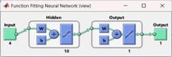
The task of anticipating the second structure can be viewed as a pattern recognition challenge, wherein the network is trained to identify the structural condition of the remaining segments observed within the sliding window. In Appendix 5, you can find the code for implementing a neural network for pattern recognition. This network utilizes the input and output matrices specified earlier and incorporates a hidden layer consisting of three nodes. The network is composed of three layers, as depicted in Figure 1 [24]. The initial layer serves as the input for the system, comprising a sequence of amino acids. The second layer acts as a hidden layer, performing prediction computations. Finally, the third layer represents the system’s output, presenting the displayed predicted secondary structure.
Figure 1. Three-tier predictive system model, input (sequence of amino acids), computational for prediction, output (predicted secondary structure)
3.4 Neural network training
The training of the pattern recognition network is based on the default scaled dual-gradient algorithm, although alternative algorithms are also accessible. During every training iteration, the training sequence is introduced to the network using the aforementioned sliding window technique. Algorithm 1 shows the steps of building and training the neural network model, which is described in detail below [25-27].
|
Algorithm 1. Learning process of proposed neural network |
|
1. Input: RostSander Dataset $X \in R^{I_1 I_2 \cdots I_N \times I_M}$ 2. [XTrain, YTrain] = Train4DArrayData; 3. [XTest, YTest] = Test4DArrayData; 4. Model Construction: 5. layers = [ imageInputLayer([28 28 1]) fullyConnectedLayer(128) reluLayer fullyConnectedLayer(64) reluLayer fullyConnectedLayer(10) softmaxLayer classificationLayer]; 6. Parameter Settings: 7. options = trainingOptions('adam', ... 'InitialLearnRate', 0.001, ... 'MaxEpochs', 10, ... 'MiniBatchSize', 32, ... 'ValidationData', {XTest, YTest}, ... 'Plots', 'training-progress'); 8. Forward Propagation: 9. net = trainNetwork(XTrain, YTrain, layers, options); 10. Model Evaluation: 11. YPred = classify(net, XTest); 12. Back propagation |
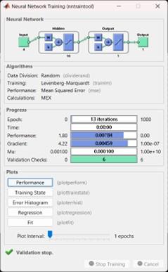
Constant evaluation of an element occurs at every given moment. The hidden units analyze the incoming signals from the input layer and produce an output signal, which resembles the firing of a neuron, by applying the logsig transfer function. The weights of the units are adjusted to minimize the difference between the obtained output and the desired output specified in the target matrix. For the actual code, please consult Attachment 7. Throughout the training process, a training tool window is launched, as depicted in Figure 2, and this particular window showcases the ongoing progress. The training showcases various aspects such as the algorithm used, performance metrics measured, the type of error taken into account, and more [28-30].
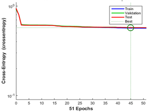
The function called “plotperform” allows you to visualize the errors encountered during the training process, including training, validation, and test errors. By running the specified commands, you can view a graphical representation of these errors in Figures 3-7.
Figure 2. The training and display tool window for the details of the training cycle and implementation execution in MATLAB
Figure 3. The plot function displays the training trend. It can be seen that in epoch 45 is the point of convergence of different lines
Figure 4. The representation of the validation process
The training process is halted when any of the specified conditions are met. For instance, in the mentioned training (net.trainparam), if the validation errors surpass a predetermined threshold over a certain number of iterations or reach the maximum permissible count of 1000, as outlined in Attachment 9, the training process is terminated.
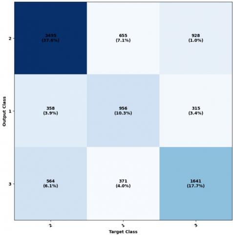
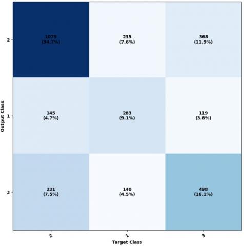
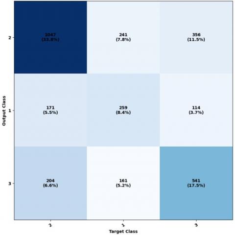
In order to analyze the response of the network, we assess the network’s outputs and compare them to the anticipated results (targets). This evaluation is performed through the examination of the confusion matrix. By studying this matrix, we can gain insights into the network’s performance and identify any discrepancies or errors in its predictions.
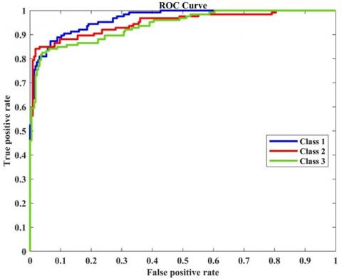
The diagonal cells represent the count of accurately categorized elements for every structural class. This displays the cells obtained from various unclassified positions, where some positions, such as Helix, have been mistakenly predicted as the coil. The cells colored in blue represent the percentage of accurately predicted elements (shown in green), while the percentage of incorrectly predicted elements is indicated by red-colored cells. We can analyze the ROC curve and a graphical representation of the true positive rate compared to the false positive rate. This analysis can be done using the provided code, and the results are illustrated in Figure 6.
Figure 5. Ownership matrix and its comparison with network output
Figure 6. Receiver Operating Characteristic (ROC) curve
(a) Test confusion matrix
(b) All confusion matrix
(c) Training confusion matrix
(d) Validation confusion matrix
Figure 7. Utilization of ownership matrix in educational subsets, validation, and testing
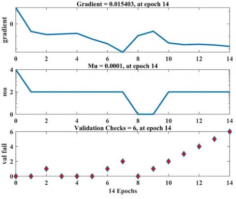
The RostSander Dataset is divided into three subcategories, considering the preferences for A-Helix, B-sheet, and coil, in order to identify proteins that include E. These proteins were not previously predicted using the previous method. It is clear that the training speed remains stable. Subsequently, we generated a new graph of the “plotperform” function and noticed that the training pattern remains consistent, albeit with a gentler slope, as depicted in Figure 8.
To illustrate the validation, we depict Figure 9. Furthermore, the potential number of errors remains unchanged under these circumstances, similar to the previous situation.
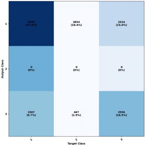
Figure 10 illustrates the ownership matrix, highlighting the variation from Figure 10, specifically in the second row and second column, which corresponds to the structural class E.
In the dataset, the item located at the intersection of the second column and second row, represented by zero, can be classified with a 10% E accuracy. Figure 11 was created to showcase the properties of the receptor agent and illustrate the relationship between the actual positive rate and the false positive rate. By comparing it to Figure 11, we can see that Classes 1, 2, and 3 exhibit noticeable proximity to one another, indicating their closeness as classes.
Figure 8. The plot function illustrates the training trend. The best result is obtained in epoch 13 with 0.3048% accuracy
Figure 9. Validation process visualization
Figure 10. Ownership matrix and its comparison with network output
Figure 11. Receiver operating characteristic (ROC) curve
In this work, 70% of the samples were utilized to train the classification model, and 15% of the dataset's samples were used for each of the validation and test phases. The outcomes are also assessed using the F1-score, accuracy, precision, and recall criteria (Eqs. (1)-(4)).
Accuracy $=\frac{T P+T N}{T P+T N+F P+F N}$ (1)
Precision $=\frac{T P}{(T P+F P)}$ (2)
Recall $=\frac{T P}{T P+F N}$ (3)
F1-Score $=2 \times \frac{\text { Precision } \times \text { Recall }}{\text { Precision }+ \text { Recal }}$ (4)
In this part, the performance of the proposed method is checked on the RostSander Dataset. For this purpose, the neural network model is built with and without regularization. Table 1 shows the results obtained for the two phases of training and testing for these two modes of reporting. The results of this table are reported based on four precision, recall, F1-score and accuracy evaluation criteria. As can be seen, the proposed neural network model with regularization has obtained better results. For example, it has achieved 98.42% precision, 98.01% recall, 97.55% F1-score and 98.15% accuracy in the training phase. Also, in the test phase, it has achieved 97.02% precision, 96.13% recall, 96.57% F1-score and 97.38% accuracy. Therefore, in the next part where the comparisons are made, the same model with regularization is used.
The proposed approach was contrasted with previously published efforts in the RostSander dataset sample classification. Table 2 lists previous studies that make use of deep learning techniques. A CNN+LSTM classifier was utilized by Du et al. [31] to categorize seven types of proteins in RostSander dataset. A distinct component for categorization based on RostSander dataset was added by Lu et al. [32]. The study's findings for 10,436 proteins showed evaluation accuracy of 82.10%. Furthermore, Yang et al. [33] provided a Detrending+ResNet-18 approach for categorizing 10,093 cases. In the assessment section, they claimed a 88.23% accuracy rate in identifying seven different types of proteins. With more inputs, deep learning techniques like CNN have shown to perform better; as a result, the techniques in Table 2 are sophisticated and have typically respectable accuracies. The suggested approach can compete with existing classifications and shows behavior similar to classifiers built using RostSander dataset.
Table 1. The results obtained from the recognition of the model
|
Models |
Precision |
Recall |
F1-Score |
Accuracy |
|
Train Phase (Without Regularization) |
98.00% |
97.11% |
98.65% |
98.13% |
|
Train Phase (With Regularization) |
98.42% |
98.01% |
97.55% |
98.15% |
|
Test Phase (Without Regularization) |
95.53% |
97.36% |
94.94% |
94.01% |
|
Test Phase (With Regularization) |
97.02% |
96.13% |
96.57% |
97.38% |
Table 2. Comparison of proposed method with other state-of-the-arts method on the RostSander dataset
|
Reference |
Method |
Accuracy |
|
Du er al. [31] |
CNN+LSTM |
82.10% |
|
Lu et al. [32] |
ResNet-31 |
89.87% |
|
Yang et al. [33] |
XGBoost |
88.23% |
|
Zamora-Resendiz and Crivelli [34] |
CNN |
85.24% |
|
Zhang et al. [35] |
CNN+LSTM |
90.14% |
|
Zhang et al. [35] |
CNN+LSTM |
88.00% |
|
Torisi et al. [36] |
MLP |
90.12% |
|
Proposed Method |
Neural Network |
94.22% |
This approach presented here uses the structural states of nearby proteins to forecast the structural condition of a protein. Nevertheless, there exist additional constraints in forecasting the structural composition of protein components, specifically when considering the minimum length requirement for each structural element. However, it is possible to tackle these limitations in the future and find solutions to overcome them. Specifically, Helix is designated for any set of four or more consecutive elements, while the Sheet structure is allocated to any group of two or more neighbouring residues. One approach to integrating this kind of information is to create supplementary networks, where the initial network predicts the structural state based on the amino acid sequence, and the second network predicts the structural element based on the predicted structural state. However, no optimization has been conducted in this regard.
[1] Ben-Gal, I., Shani, A., Gohr, A., Grau, J., Arviv, S., Shmilovici, A., Grosse, I. (2005). Identification of transcription factor binding sites with variable-order Bayesian networks. Bioinformatics, 21(11): 2657-2666. https://doi.org/10.1093/bioinformatics/bti410
[2] Crooks, G.E., Brenner, S.E. (2004). Protein secondary structure: Entropy, correlations and prediction. Bioinformatics, 20(10): 1603-1611. https://doi.org/10.1093/bioinformatics/bth132
[3] Cuff, J.A., Barton, G.J. (1999). Evaluation and improvement of multiple sequence methods for protein secondary structure prediction. Proteins: Structure, Function, and Bioinformatics, 34(4): 508-519. https://doi.org/10.1002/(SICI)1097-0134(19990301)34:4<508:AID-PROT10>3.0.CO;2-4
[4] Durbin, R., Eddy, S.R., Krogh, A., Mitchison, G. (1998). Biological sequence analysis: Probabilistic models of proteins and nucleic acids. Cambridge University Press.
[5] Fischer, D., Eisenberg, D. (1996). Protein fold recognition using sequence-derived predictions. Protein Science, 5(5): 947-955. https://doi.org/10.1002/pro.5560050516
[6] Ouali, M., King, R.D. (2000). Cascaded multiple classifiers for secondary structure prediction. Protein Science, 9(6): 1162-1176. https://doi.org/10.1110/ps.9.6.1162
[7] Siermala, M., Juhola, M., Vihinen, M. (2001). On preprocessing of protein sequences for neural network prediction of polyproline type II secondary structures. Computers in Biology and Medicine, 31(5): 385-398. https://doi.org/10.1016/S0010-4825(01)00013-0
[8] Pollastri, G., Przybylski, D., Rost, B., Baldi, P. (2002). Improving the prediction of protein secondary structure in three and eight classes using recurrent neural networks and profiles. Proteins: Structure, Function, and Bioinformatics, 47(2): 228-235. https://doi.org/10.1002/prot.10082
[9] Costantini, S., Colonna, G., Facchiano, A.M. (2006). Amino acid propensities for secondary structures are influenced by the protein structural class. Biochemical and Biophysical Research Communications, 342(2): 441-451. https://doi.org/10.1016/j.bbrc.2006.01.159
[10] Aydin, Z., Altunbasak, Y., Borodovsky, M. (2006). Protein secondary structure prediction for a single-sequence using hidden semi-Markov models. BMC Bioinformatics, 7: 1-15. https://doi.org/10.1186/1471-2105-7-178
[11] Reyaz-Ahmed, A., Zhang, Y.Q. (2007). Protein secondary structure prediction using genetic neural support vector machines. In 2007 IEEE 7th International Symposium on BioInformatics and BioEngineering, Boston, MA, USA, pp. 1355-1359. https://doi.org/10.1109/BIBE.2007.4375746
[12] Babaei, S., Seyyedsalehi, S.A., Geranmayeh, A. (2008). Pruning neural networks for protein secondary structure prediction. In 2008 8th IEEE International Conference on BioInformatics and BioEngineering, Athens, Greece, pp. 1-6. https://doi.org/10.1109/BIBE.2008.4696702
[13] Zhou, Z., Yang, B., Hou, W. (2010). Association classification algorithm based on structure sequence in protein secondary structure prediction. Expert Systems with Applications, 37(9): 6381-6389. https://doi.org/10.1016/j.eswa.2010.02.081
[14] Babaei, S., Geranmayeh, A., Seyyedsalehi, S.A. (2010). Protein secondary structure prediction using modular reciprocal bidirectional recurrent neural networks. Computer Methods and Programs in Biomedicine, 100(3): 237-247. https://doi.org/10.1016/j.cmpb.2010.04.005
[15] Madera, M., Calmus, R., Thiltgen, G., Karplus, K., Gough, J. (2010). Improving protein secondary structure prediction using a simple k-Mer model. Bioinformatics, 26(5): 596-602. https://doi.org/10.1093/bioinformatics/btq020
[16] Yang, B., Wu, Q., Ying, Z., Sui, H. (2011). Predicting protein secondary structure using a mixed-modal SVM method in a compound pyramid model. Knowledge-Based Systems, 24(2): 304-313. https://doi.org/10.1016/j.knosys.2010.10.002
[17] Yang, B., Qu, W., Xie, Y., Zhai, Y. (2011). Predicting protein second structure using a novel hybrid method. Expert Systems with Applications, 38(9): 11657-11664. https://doi.org/10.1016/j.eswa.2011.03.045
[18] Babaei, S., Geranmayeh, A., Seyyedsalehi, S.A. (2012). Towards designing modular recurrent neural networks in learning protein secondary structures. Expert Systems with Applications, 39(6): 6263-6274. https://doi.org/10.1016/j.eswa.2011.12.059
[19] Zangooei, M.H., Jalili, S. (2012). Protein secondary structure prediction using DWKF based on SVR-NSGAII. Neurocomputing, 94: 87-101. https://doi.org/10.1016/j.neucom.2012.04.015
[20] Liang, L. (2012). Predicting the secondary structure of proteins using new ways of classification. In 2012 4th International Conference on Intelligent Human-Machine Systems and Cybernetics, Nanchang, China, pp. 212-215. https://doi.org/10.1109/IHMSC.2012.147
[21] Fayech, S., Essoussi, N., Limam, M. (2013). Data mining techniques to predict protein secondary structures. In 2013 5th International Conference on Modeling, Simulation and Applied Optimization (ICMSAO), Hammamet, Tunisia, pp. 1-5. https://doi.org/10.1109/ICMSAO.2013.6552701
[22] Shamima, B., Savitha, R., Suresh, S., Saraswathi, S. (2013). Protein secondary structure prediction using a fully complex-valued relaxation network. In The 2013 International Joint Conference on Neural Networks (IJCNN), Dallas, TX, USA, pp. 1-8. https://doi.org/10.1109/IJCNN.2013.6707126
[23] Hulianytskyi, L.F., Rudyk, V.O. (2013). Protein structure prediction problem: Formalization using quaternions. Cybernetics and Systems Analysis, 49: 597-602. https://doi.org/10.1007/s10559-013-9546-8
[24] Patel, M.S., Mazumdar, H.S. (2014). Knowledge base and neural network approach for protein secondary structure prediction. Journal of Theoretical Biology, 361: 182-189. https://doi.org/10.1016/j.jtbi.2014.08.005
[25] Prošková, J. (2014). Description of protein secondary structure using dual quaternions. Journal of Molecular Structure, 1076: 89-93. https://doi.org/10.1016/j.molstruc.2014.07.031
[26] Li, B., Li, Y., Gong, L. (2014). Protein secondary structure optimization using an improved artificial bee colony algorithm based on AB off-lattice model. Engineering Applications of Artificial Intelligence, 27: 70-79. https://doi.org/10.1016/j.engappai.2013.06.010
[27] Tan, Y.T., Rosdi, B.A. (2015). FPGA-based hardware accelerator for the prediction of protein secondary class via fuzzy K-nearest neighbors with Lempel–Ziv complexity based distance measure. Neurocomputing, 148: 409-419. https://doi.org/10.1016/j.neucom.2014.06.001
[28] Zhang, L., Zhao, X., Kong, L., Liu, S. (2014). A novel predictor for protein structural class based on integrated information of the secondary structure sequence. Biochimie, 103: 131-136. https://doi.org/10.1016/j.biochi.2014.05.008
[29] Dorn, M., e Silva, M.B., Buriol, L.S., Lamb, L.C. (2014). Three-dimensional protein structure prediction: Methods and computational strategies. Computational Biology and Chemistry, 53: 251-276. https://doi.org/10.1016/j.compbiolchem.2014.10.001
[30] Kong, L., Zhang, L., Lv, J. (2014). Accurate prediction of protein structural classes by incorporating predicted secondary structure information into the general form of Chou's pseudo amino acid composition. Journal of Theoretical Biology, 344: 12-18. https://doi.org/10.1016/j.jtbi.2013.11.021
[31] Du, X., Sun, S., Hu, C., Yao, Y., Yan, Y., Zhang, Y. (2017). DeepPPI: Boosting prediction of protein–protein interactions with deep neural networks. Journal of Chemical Information and Modeling, 57(6): 1499-1510. https://doi.org/10.1021/acs.jcim.7b00028
[32] Lu, W., Wu, Q., Zhang, J., Rao, J., Li, C., Zheng, S. (2022). Tankbind: Trigonometry-aware neural networks for drug-protein binding structure prediction. Advances in Neural Information Processing Systems, 35: 7236-7249.
[33] Yang, H., Xiong, Z., Zonta, F. (2022). Construction of a deep neural network energy function for protein physics. Journal of Chemical Theory and Computation, 18(9): 5649-5658. https://doi.org/10.1021/acs.jctc.2c00069
[34] Zamora-Resendiz, R., Crivelli, S. (2019). Structural learning of proteins using graph convolutional neural networks. BioRxiv, 610444. https://doi.org/10.1101/610444
[35] Zhang, L., Yu, G., Xia, D., Wang, J. (2019). Protein–protein interactions prediction based on ensemble deep neural networks. Neurocomputing, 324: 10-19. https://doi.org/10.1016/j.neucom.2018.02.097
[36] Torrisi, M., Kaleel, M., Pollastri, G. (2019). Deeper profiles and cascaded recurrent and convolutional neural networks for state-of-the-art protein secondary structure prediction. Scientific Reports, 9(1): 12374. https://doi.org/10.1038/s41598-019-48786-x