Arif Setiawan* | Hadiyanto Hadiyanto | Catur E. Widodo
© 2022 IIETA. This article is published by IIETA and is licensed under the CC BY 4.0 license (http://creativecommons.org/licenses/by/4.0/).
OPEN ACCESS
Camera is the main tool for monitoring shrimp underwater with a noninvasive method. Distance of the shrimp underwater with the varying camera causes the monitoring of the estimated shrimp size to be less accurate. This study provides a new solution to detect the distance of shrimp underwater with a camera using the Euclidian distance and triangle similarity algorithm. The problem raised in this study is how to measure the distance of a shrimp underwater with a camera. The method used has several stages, including using the grayscale image method, image thresholding, edge detection, detection of Region of Interest (ROI), determining the position of shrimp coordinates, calculating the length of shrimp coordinates, camera calibration using the triangle similarity algorithm, calculating the estimated distance of shrimp with the camera. The study results obtained a focal length value of 1298.58, the value of the distance between the shrimp and the camera (D') for 5 positions of shrimp underwater from 50 cm – 19.86 cm, and the RE value from 0% - 0.13%. In conclusion, this method can be used to measure the estimated distance between of moving shrimp and a camera with a low error rate.
shrimp, underwater, distance estimation, Euclidian distance, triangle similarity
Shrimp farming is a business in the waters sector that has an impact on economic improvement in many developing countries [1]. Shrimp is a cultivated product that is very popular with people in many countries [2]. Shrimp results can be processed into various processed foods. Shrimp is one component of food security [3]. Monitoring the condition of shrimp under water is very much needed in aquaculture [4]. Monitoring the size of shrimp from seed to harvest is needed to determine feed requirements [5]. The increasing demand for shrimp causes shrimp farmers to provide abundant harvests. Non-invasive monitoring methods using the camera are needed for monitoring shrimp underwater, because traditional monitoring methods with direct shrimp catch models, cause shrimp stress and death, thereby reducing crop yields [6].
Computer vision is a modern technology that is suitable to be applied in the shrimp farming environment [7]. Smart shrimp farming uses computer vision technology, using cameras as a medium for monitoring shrimp under water [8].
The position of the shrimp that swims freely underwater causes the monitoring of shrimp size to be inaccurate [9]. The difference in the position of the shrimp with the distance of the shrimp object with the camera varies, causing the shrimp captured by the camera in the form of a 2D image to have an inaccurate size [10]. A method is needed to determine the estimated distance of the position of shrimp underwater with a camera, so that from the estimated distance obtained, it can be used to increase the accuracy of monitoring shrimp size [11].
Digital image processing is the first step in computer vision in detecting shrimp under water [12]. Image segmentation technique is used to process the digital image of shrimp. Changing the red green blue (RGB) image to grayscale is the first step in segmentation. Thresholding is a method that is widely used for digital image segmentation. Thresholding is the stage of separating the image object from the background and foreground objects [13]. Edge detection is the stage for detecting objects after the thresholding process. In this operation, the edges of objects are detected to make the boundary between foreground and background clearer [11]. Canny algorithm is the most widely used method in edge detection [14]. This method has a good level of accuracy in providing a border on an image [15].
Region of Interest (ROI) detection is used to retrieve the object area from its background [16]. ROI detection is used to predict the object area in a digital image [17]. After the image object area is known through the ROI process, the coordinates of the object area point are calculated. Image object is an area in the image which is a pixel matrix. Image objects have position coordinates that can be known from the coordinates of the X and Y axes in the 2D image dimensions [18].
Triangle similarity is widely used in several research fields. Spirkovska in his research proposed the introduction of 3D objects using similar triangles and decision tree algorithms. Spirkovska uses similar triangles algorithm to calculate the similarity of object characteristics and decision tree algorithm to classify objects [19]. Madi in his research proposes to determine the distance in the recognition of deformed 3D objects using triangles decomposition. Madi explained that the resulting graph distance estimate is error tolerant, so this algorithm is very suitable to be used [20].
Klinaku in his research proposed a similar triangle for the distance property on the doppler effect. In his research, my clinic used the Euclidian distance from the doppler effect to calculate the frequency of the waves [21]. Hu in his research used a similar triangle to reconstruct a map to explore information on flexibility and scalability in 3 dimensions (3D). Hu processed the digital image of the map by determining the appropriate object plane in terms of similarity, texture smoothness, and image boundaries [22].
In his research, Bundak uses a similar triangle for positioning in magnetic field space. Bundak uses a combination of fuzzy, similar triangle and Euclidian distance to estimate the position in the force field area in a magnetic field [23]. Garg in his research proposed a new algorithm for measuring distance in fuzzy clustering using a triangle center. Grag explained that there are 4 central points in clustering, namely the centroid, orthocenter, circumcenter and incenter of the triangle. Garg uses these 4 types of center points to determine distance [24]. Navarro in his research proposed a similar triangle to detect anomalies. Navarro explained that triangle-based detection is included in distance-based detection. This study resulted in a good system for outlier detection [25].
The researchers observed shrimp, regardless of the distance between the fish and shrimp and the camera. Liu in his research carried out shrimp detection using the deep learning shrimpnet 3 algorithm [26]. Lin in his research conducted shrimp detection using the Yolo algorithm, Lin explained that the brightness and light distribution factors were very influential in the detection of shrimp [27]. Another study was conducted by Isa, using CNN transfer learning to observe shrimp under water. Isa used the Over Union Intersection (IOU) method to analyze the image [28]. Hu in his research made observations to recognize patterns and classify shrimp, Hu explained that in observing shrimp patterns using the CNN Shrimpnet algorithm [29]. Yu in his research made observations on shrimp diseases. Yu explained that his research looked at the bacteria found in shrimp as seen from the Total Variable Count (TVC) [30]. In his research, Thai observed population density and shrimp size, Thai used computer vision method with U-net and watershed segmentation methods [31].
From the background, there is no application of the similar triangle algorithm for distance detection to objects, this study proposes a similar triangle method to detect the distance of shrimp underwater with a camera.
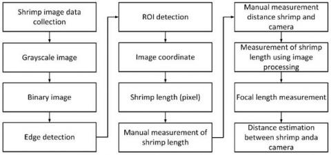
This research has several stages, the stages of research carried out are (a) data retrieval of shrimp, (b) processing of RGB shrimp images into grayscale images, (c) processing of grayscale images into binary images using the Otsu algorithm, (d) detecting the ROI of shrimp objects, (e) processing the coordinates of the shrimp position, (f) calculating the length of the shrimp underwater from the camera catch, (g) measuring the length of the shrimp manually with a measuring instrument, (h) measuring the estimated distance between the shrimp and the camera manually, (i) calculate the focal length value, (j) measure the estimated distance between the shrimp underwater and the camera from 5 positions to 1 shrimp. The research flow can clearly be seen in Figure 1.
Figure 1. Research flowchart
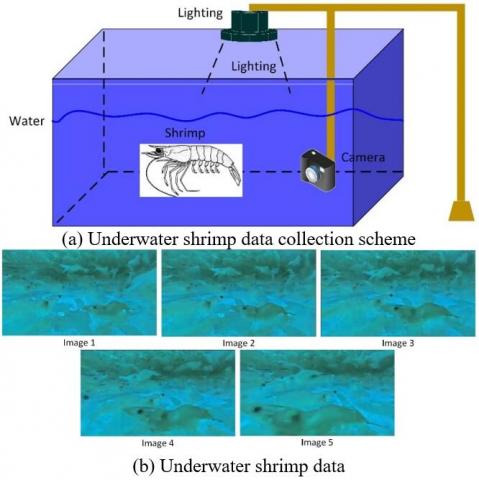
The data used in this study using data on shrimp underwater. The process of taking data using a camera and producing a video file. From the video obtained, it is then extracted into a jpg format image. The image with the position of the shrimp in front of the camera was chosen as research data, consisting of 5 digital images. The tool used to extract the shrimp video into an image is Python 3 and OpenCV library. OpenCV library is specifically used for image processing. The process that carried out is to read the video file, then extract it into a jpg image file. The function used to read video files is cv2.videocapture(), and the function used to convert video files into image frames is cam.read(). The 5-minute video is extracted into 6404 image frames. The files used in this study are frames to 6305, 6310, 6315, 6320, 6325.
The digital image is a 2-dimensional function, namely x and y which are spatial coordinates. Digital images represent the quantity of image elements called pixels [32]. Digital images also represent the lighting of objects taken from the camera [33]. Digital images are sent electronically which are transferred to physical storage media in the form of photos and videos [34]. Grayscale image is an image with a gray level of pixels on the image object [35]. Grayscale image is the result of processing from RGB image, with the same red green blue value [36].
A binary image is an image with a pixel value of 0 and 1. The thresholding technique is used for the binary process [37]. Binary images are used to separate objects from their backgrounds [38]. Edge detection is an approach to contour detection, which aims to measure the presence of object area boundaries in certain images [39]. Canny algorithm is one of the algorithms used for edge detection [40]. Canny processes the image using a gaussian filter [41]. The Canny algorithm detects edges in an image by eliminating noise around the object [17].
Euclidean distance is a method for measuring the distance from 2 points. This method is the development of the Pythagorean method [42]. Euclidian distance can be applied to both 2D and 3D objects. the application of Euclidian distance to 2D objects is applied to digital images, namely the calculation of the distance between the initial coordinates (ax,ay) and the final coordinates (bx,by) [43]. Euclidian distance equation is calculated using Eq. (1) [44].
$d(a, b)=\sqrt{(b x-a x)^2+(b y-a y)^2}$ (1)
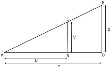
Triangle similarity is 2 triangles that have the same shape, but different sizes. Two triangles that have the same shape have the same angles in each triangle [21]. The 2D triangle in the image must not overlap, this triangle is 2 different planes [22]. Triangles similarity is shown in Figure 2 and the triangle similarity equation is shown in Eqns. (2) and (3) [45].
$\angle C A B=\angle E A D$ (2)
$\frac{A B}{A D}=\frac{C B}{E D}$ (3)
Figure 2. Triangle similarity ABC-ADE
Focal length is the distance between the lens and the image object on the camera. Focal length is measured in millimeters (mm). Focal length is a lens parameter on the camera that shows the image object [46]. Focal length is the distance between the optical center and the camera sensor, which is used to adjust the focus of the image captured by the camera [47]. Focal length adjusts the focus by adjusting the optical center distance so that incoming light can sharpen the image on the camera [48]. The equation for calculating the focal length is shown in Eq. (4), and for calculating distance estimation shrimp underwater and camera shown in equation 5. Where P is the length of the object captured by the camera in pixels, W is the original length of the object, D is the original distance from the object to the camera, P' is the new length of the object captured by the camera in pixels and D' is distance estimation between object and camera.
$F=(P * D) / W$ (4)
$D^{\prime}=(W * F) / P^{\prime}$ (5)
The evaluations used for image processing are Structural Similarity Index Measure (SSIM), Peak Signal Noise Ratio (PSNR) and Mean Squared Error (MSE). The value of each is calculated using the Eqns. (6)-(8) [49].
$\frac{\left(2 \mu_x \mu_y+c_1\right)\left(2 \sigma_{x y}+c_2\right)}{\left(\mu_x^2+\mu_y^2+c_1\right)\left(\sigma_x^2+\sigma_y^2+c_2\right)}$ (6)
$P S N R=10 \cdot \log _{10} f(x)=\left(\frac{M A X_1^2}{M S E}\right)$ (7)
$M S E=\frac{1}{n}\left|x-x^{\prime}\right|^2=\frac{1}{n} \sum_{i=1}^n\left(x-x^{\prime}\right)^2$ (8)
The error evaluation is calculated using the relative error (RE) value. The RE value and percent error is calculated from the Eqns. (9) and (10) [50].
$R E=\frac{ { measure }- { real }}{ { real }}$ (9)
Percent Error $=\frac{{ measure }- { real }}{ { real }} \times 100 \%$ (10)
Shrimp data is taken from a shrimp culture pond, the data taken is video in mp4 format. From video data then extracted into image frames digital jpg format. Schematic drawing for shrimp data acquisition is shown in Figure 3 (a). The research was implemented using 5 digital images of underwater shrimp taken from observations of 1 shrimp underwater. 5 digital images of shrimp are 5 positions of 1 shrimp. The detailed shrimp image data is shown in Figure 3 (b).
Figure 3. Data collection
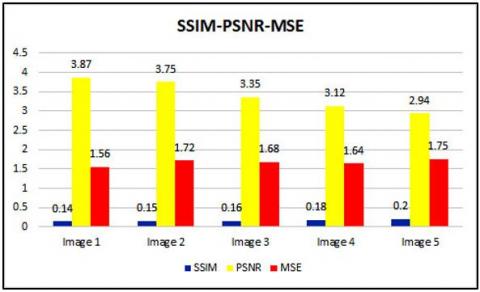
The experiment begins by converting an RGB image into an image grayscale and binary images. The process of changing to a binary image uses a threshold value of 0.01 and uses the Otsu algorithm. At this stage, the shrimp object is separated from the background. At this stage, morphological and dilation processes are also carried out. The morphology process is used to reduce noise in the digital shrimp image, and the dilation process is useful for the binary image thickening process. The experimental results show that the shrimp object has a white value of pixel 1, and the background value of pixel 0 is black. From the results of this experiment, the value of the Structural Similarity Index SSIM for 5 shrimp images, namely the value of SSIM 1=0.14, SSIM 2=0.15, SSIM 3 = 0.16, SSIM 4=0.18, SSIM 5=0.2. In detail, the SSIM value for the thresholding process is shown in Figure 4 (a).
The experiment continued with the edge detection process. In this study the algorithm used is canny. The experiment was carried out on 5 digital images. From this stage, the edge of the digital image of the shrimp is obtained as a barrier between the shrimp object and its background. Evaluation of canny edge detection using Peak Signal Noise Ratio (PSNR) and Mean Sequare Error (MSE). The values obtained for PSNR are PSNR 1=3.87, PSNR 2=3.75, PSNR 3=3.35, PSNR 4=3.12, PSNR 5=2.9. And the MSE value obtained is MSE 1=1.56, MSE 2=1.72, MSE 3 = 1.68, MSE 4=1.64, MSE 5=1.75. In detail the PSNR and MSE values of the thresholding process are shown in Figure 4 (a).
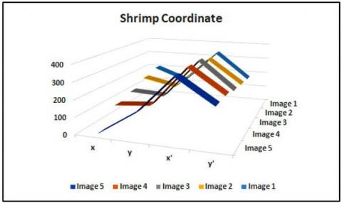
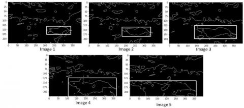
The experiment was continued at the ROI detection stage. This step is used to clarify the detected shrimp object. The shrimp object that is obtained is given a box frame border as an object marker. At this stage, the coordinates of the box frame of the digital shrimp image are also obtained. The coordinates obtained are the top left point symbolized by (x,y) and the bottom right point symbolized by (x',y') for the 5 positions of the shrimp objects underwater. The coordinates obtained are image 1 (x,y)=(208,132) (x',y')=(340,176), image 2 (x,y)=(179,135), (x',y') (335,186), image 3 (x,y)=(136,126), (x',y')=(365,198), image 4 (x,y)=(105,124), (x',y')=(357.224), image 5 (x,y)=(0.139), (x',y')=(361,224).
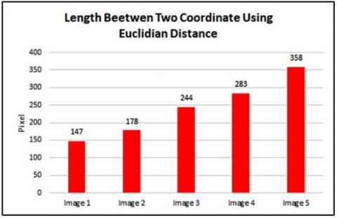
From the results of these coordinate points, the length (P) between the 2 coordinate points in the shrimp object is obtained in pixel units. The measurement method is to calculate the distance of the pixel points using the Euclidian distance. The calculation process uses Eq. (1). The length of the shrimp object obtained is P1=147 pixels, P2=178 pixels, P3=244 pixels, P4=283 pixels, P5=358 pixels. In detail the coordinates and the length of the 2 coordinate points of each image are shown in Table 1, and Figures 4 (b) and (c).
From the coordinates of the shrimp position, a box frame is made as a shrimp marker. This box frame is 5 positions of 1 shrimp. In detail, the results of ROI detection and box frames for shrimp images are shown in Figure 5. From the results of this experiment, it can be seen that the closer the shrimp is to the camera, the bigger the shrimp will be.
(a) Value of SSIM, PSNR, MSE
(b) Coordinates of 5 shrimp image
(c) Length of two points coordinate
Figure 4. Error value, coordinate and length coordinate
Figure 5. Detecting the shrimp underwater using ROI
Table 1. Coordinates the position of the shrimp underwater
|
Image |
Top left coordinates |
Bottom right coordinate |
Length between 2 coordinate in pixel (P) |
||
|
x |
y |
x' |
y' |
||
|
Image 1 |
208 |
132 |
340 |
176 |
147 |
|
Image 2 |
179 |
135 |
335 |
186 |
178 |
|
Image 3 |
136 |
126 |
365 |
198 |
244 |
|
Image 4 |
105 |
124 |
367 |
224 |
283 |
|
Image 5 |
0 |
139 |
361 |
224 |
358 |
The experiment continued with manual measurement of live shrimp. This step is carried out to calibrate the size of live shrimp in centimeters (cm) with the size of the shrimp ROI detection results in pixels. The measurement method was carried out by catching 1 shrimp and measuring it with a measuring instrument manually. From the measurement results, it was found that the length of the shrimp was 5.6 cm, as shown in Figure 6 (a).
The next experiment is camera calibration. This calibration process uses the Triangle Similarity (TS) algorithm. This stage aims to factor correction between the size of the shrimp ROI results with the size of the original shrimp. From the TS algorithm, the focal length value is obtained. Focal length is a parameter for camera calibration. The schematic of the TS process is depicted in Figure 6 (b). From the computational calibration results, the focal length value is 1298. 58. This calculation process uses Eq. (4).
Figure 6. Focal length calculation
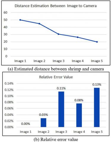
Table 2. Estimated distance between shrimp and the camera
|
Image |
Distance Estimation (D')(cm) |
Difference between estimated and fix value (cm) |
Relative error value (RE) |
|
Image 1 |
50 |
0 |
0.00% |
|
Image 2 |
44.82 |
0.01 |
0.03% |
|
Image 3 |
30.63 |
0.04 |
0.11% |
|
Image 4 |
26.25 |
0.02 |
0.08% |
|
Image 5 |
19.86 |
0.03 |
0.13% |
Figure 7. Estimated distance and relative error value
The experiment was continued in the process of calculating the distance between the shrimp and the camera. This process is calculated using Eq. (5). From the position of 1 shrimp that swims freely in front of the camera obtained 5 distances of shrimp with the camera. The process of calculating the distance between the camera and shrimp underwater uses the formula 2.5. The estimated distance values (D') detected are D1'=50 cm, D2'=44.82 cm, D3'=30.63 cm, D4'=26.25 cm, D5'=19.86 cm. From these 5 detected distances, the Relative Error (RE) value is obtained, the RE calculation process uses Eq. (10). RE values obtained are RE1=0%, RE2=0.03%, RE3=0.11%, RE4=0.08%, RE5=0.13%. In detail, the estimated distance between shrimp and camera is shown in Table 2 and Figure 7 (a), the RE value is shown in Table 2 and Figure 7 (b).
Based on the results of the study, it can be concluded that the measurement of the estimated distance of the shrimp moving underwater with the camera gets 5 different distances, namely D1'=50 cm, D2'=44.82 cm, D3'=30.63 cm, D4'=26.25 cm, D5'=19.86 cm. From this distance the relative error values obtained are RE1=0%, RE2=0.03%, RE3=0.11%, RE4=0.08%, RE5=0.13%. This conclude that the Euclidian distance and triangles similarity algorithms can be used to measure the estimated distance of moving shrimp using a camera with a low error rate. Future research is using the estimated distance of the shrimp with the camera as one of the variables to calculate the size of the shrimp underwater using machine learning.
This research was supported by the Doctoral program of Information Systems, School of Postgraduate Studies, Diponegoro University, and Information Systems Study Program, Muria Kudus University.
|
d |
Euclidian distance |
|
F |
Focal length, mm |
|
P |
Length between 2 image coordinates, pixels |
|
D |
The original length of the shrimp object, cm |
|
W |
Shrimp's original distance to the camera |
|
D’ |
Estimated distance of shrimp to camera |
|
PSNR |
Peak signal noise ratio |
|
MSE |
Mean square error |
|
RE |
Relatif Error |
|
MAX |
Maximum pixel value of the image |
|
Greek symbols |
|
|
σ |
Variance x and y |
|
µ |
Average of x and y |
|
Subscripts |
|
|
x, y |
Image dimensions |
[1] Ray, S., Mondal, P., Paul, A.K., Iqbal, S., Atique, U., Islam, M.S., Mahboob, S., Al-Ghanim, K.A., Al-Misned, F., Begum, S. (2021). Role of shrimp farming in socio-economic elevation and professional satisfaction in coastal communities. Aquaculture Reports, 20: 100708. https://doi.org/10.1016/j.aqrep.2021.100708
[2] Priadana, A., Murdiyanto, A.W. (2020). Klasterisasi udang berdasarkan ukuran berbasis pemrosesan citra digital menggunakan metode CCA dan DBSCAN. Jurnal Teknologi dan Sistem Komputer, 8(2): 106-112. https://doi.org/10.14710/jtsiskom.8.2.2020.106-112
[3] Liu, Z. (2020). Soft-shell shrimp recognition based on an improved AlexNet for quality evaluations. Journal of Food Engineering, 266: 109698. https://doi.org/10.1016/j.jfoodeng.2019.109698
[4] Yang, X., Zhang, S., Liu, J., Gao, Q., Dong, S., Zhou, C. (2021). Deep learning for smart fish farming: applications, opportunities and challenges. Reviews in Aquaculture, 13(1): 66-90. https://doi.org/10.1111/raq.12464
[5] Rashid, M., Nayan, A.A., Rahman, M., Simi, S.A., Saha, J., Kibria, M.G. (2022). IoT based smart water quality prediction for biofloc aquaculture. arXiv preprint arXiv:2208.08866. https://doi.org/10.14569/IJACSA.2021.0120608
[6] Liu, Z., Jia, X., Xu, X. (2019). Study of shrimp recognition methods using smart networks. Computers and Electronics in Agriculture, 165: 104926. https://doi.org/10.1016/j.compag.2019.104926
[7] Ubina, N., Cheng, S.C., Chang, C.C., Chen, H.Y. (2021). Evaluating fish feeding intensity in aquaculture with convolutional neural networks. Aquacultural Engineering, 94: 102178. https://doi.org/10.1016/j.aquaeng.2021.102178
[8] Liu, H., Liu, T., Gu, Y., Li, P., Zhai, F., Huang, H., He, S. (2021). A high-density fish school segmentation framework for biomass statistics in a deep-sea cage. Ecological Informatics, 64: 101367. https://doi.org/10.1016/j.ecoinf.2021.101367
[9] Ihsanario, A., Ridwan, A. (2021). Optimal feeding frequency on the growth performance of whiteleg shrimp (Litopenaeus vannamei) during grow-out phase. 3BIO J. Biol. Sci. Technol. Manag., 3(1): 42–55. http://journals.itb.ac.id/index.php/3bio/article/view/16120
[10] Zhang, L., Wang, J., Duan, Q. (2020). Estimation for fish mass using image analysis and neural network. Computers and Electronics in Agriculture, 173: 105439. https://doi.org/10.1016/j.compag.2020.105439
[11] Swamidoss, I.N., Amro, A.B., Sayadi, S. (2021). Systematic approach for thermal imaging camera calibration for machine vision applications. Optik, 247: 168039. https://doi.org/10.1016/j.ijleo.2021.168039
[12] Trivedi, J.D., Mandalapu, S.D., Dave, D.H. (2022). Vision-based real-time vehicle detection and vehicle speed measurement using morphology and binary logical operation. Journal of Industrial Information Integration, 27: 100280. https://doi.org/10.1016/j.jii.2021.100280
[13] Xu, W., Chen, H., Su, Q., Ji, C., Xu, W., Memon, M.S., Zhou, J. (2019). Shadow detection and removal in apple image segmentation under natural light conditions using an ultrametric contour map. Biosystems Engineering, 184: 142-154. https://doi.org/10.1016/j.biosystemseng.2019.06.016
[14] Al-Musawi, A.K., Anayi, F., Packianather, M. (2020). Three-phase induction motor fault detection based on thermal image segmentation. Infrared Physics & Technology, 104: 103140. https://doi.org/10.1016/j.infrared.2019.103140
[15] Hossain, M.S., Yasir, M., Wang, P., Ullah, S., Jahan, M., Hui, S., Zhao, Z. (2021). Automatic shoreline extraction and change detection: A study on the southeast coast of Bangladesh. Marine Geology, 441: 106628. https://doi.org/10.1016/j.margeo.2021.106628
[16] Delwiche, S.R., Baek, I., Kim, M.S. (2021). Does spatial region of interest (ROI) matter in multispectral and hyperspectral imaging of segmented wheat kernels? Biosystems Engineering, 212: 106-114. https://doi.org/10.1016/j.biosystemseng.2021.10.003
[17] Yang, Y., Zhao, X., Huang, M., Wang, X., Zhu, Q. (2021). Multispectral image based germination detection of potato by using supervised multiple threshold segmentation model and Canny edge detector. Computers and Electronics in Agriculture, 182: 106041. https://doi.org/10.1016/j.compag.2021.106041
[18] Shen, X., Hu, H., Li, X., Li, S. (2021). Study on PCA-SAFT imaging using leaky Rayleigh waves. Measurement, 170: 108708. https://doi.org/10.1016/j.measurement.2020.108708
[19] Spirkovska, L. (1993). Three-dimensional object recognition using similar triangles and decision trees. Pattern Recognition, 26(5): 727-732. https://doi.org/10.1016/0031-3203(93)90125-G
[20] Madi, K., Paquet, E., Kheddouci, H. (2019). New graph distance for deformable 3D objects recognition based on triangle-stars decomposition. Pattern Recognition, 90: 297-307. https://doi.org/10.1016/j.patcog.2019.01.040
[21] Klinaku, S., Berisha, V. (2019). The Doppler effect and similar triangles. Results in Physics, 12: 846-852. https://doi.org/10.1016/j.rinp.2018.12.024
[22] Hu, Z., Hou, Y., Tao, P., Shan, J. (2021). IMGTR: Image-triangle based multi-view 3D reconstruction for urban scenes. ISPRS Journal of Photogrammetry and Remote Sensing, 181: 191-204. https://doi.org/10.1016/j.isprsjprs.2021.09.009
[23] Bundak, C.E.A., Abd Rahman, M.A., Karim, M.K.A., Osman, N.H. (2022). Fuzzy rank cluster top k Euclidean distance and triangle based algorithm for magnetic field indoor positioning system. Alexandria Engineering Journal, 61(5): 3645-3655. https://doi.org/10.1016/j.aej.2021.08.073
[24] Garg, H., Rani, D. (2022). Novel distance measures for intuitionistic fuzzy sets based on various triangle centers of isosceles triangular fuzzy numbers and their applications. Expert Systems with Applications, 191: 116228. https://doi.org/10.1016/j.eswa.2021.116228
[25] Navarro, J., de Diego, I.M., Fernández, R.R., Moguerza, J.M. (2022). Triangle-based outlier detection. Pattern Recognition Letters, 156: 152-159. https://doi.org/10.1016/j.patrec.2022.03.008
[26] Liu, Z., Jia, X., Xu, X. (2019). Study of shrimp recognition methods using smart networks. Computers and Electronics in Agriculture, 165: 104926. https://doi.org/10.1016/j.compag.2019.104926
[27] Lin, H.Y., Lee, H.C., Ng, W.L., et al. (2019). Estimating shrimp body length using deep convolutional neural network. In 2019 ASABE Annual International Meeting (p. 1). American Society of Agricultural and Biological Engineers. https://doi.org/10.13031/aim.201900724
[28] Isa, I.S., Norzrin, N.N., Sulaiman, S.N., Hamzaid, N.A., Maruzuki, M.I.F. (2020). CNN transfer learning of shrimp detection for underwater vision system. In 2020 1st International Conference on Information Technology, Advanced Mechanical and Electrical Engineering (ICITAMEE), pp. 226-231. https://doi.org/10.1109/ICITAMEE50454.2020.9398474
[29] Hu, W.C., Wu, H.T., Zhang, Y.F., Zhang, S.H., Lo, C.H. (2020). Shrimp recognition using ShrimpNet based on convolutional neural network. Journal of Ambient Intelligence and Humanized Computing, 1-8. https://doi.org/10.1007/s12652-020-01727-3
[30] Yu, X., Yu, X., Wen, S., Yang, J., Wang, J. (2019). Using deep learning and hyperspectral imaging to predict total viable count (TVC) in peeled Pacific white shrimp. Journal of Food Measurement and Characterization, 13(3): 2082-2094. https://doi.org/10.1007/s11694-019-00129-0
[31] Thai, T.T.N., Nguyen, T.S., Pham, V.C. (2021). Computer vision based estimation of shrimp population density and size. In 2021 International Symposium on Electrical and Electronics Engineering (ISEE), pp. 145-148. https://doi.org/10.1109/ISEE51682.2021.9418638
[32] Gonzalez, R.C., Woods, R.E. (2008). CV Book, vol. 3rd Edition.
[33] Jain, A.K. (1989). Fundamentals of digital image processing. Prentice-Hall, Inc..
[34] Taoufik, N., Boumya, W., Achak, M., Chennouk, H., Dewil, R., Barka, N. (2022). The state of art on the prediction of efficiency and modeling of the processes of pollutants removal based on machine learning. Science of the Total Environment, 807: 150554. https://doi.org/10.1016/j.scitotenv.2021.150554
[35] Han, Y., Song, T., Feng, J., Xie, Y. (2021). Grayscale-inversion and rotation invariant image description with sorted LBP features. Signal Processing: Image Communication, 99: 116491. https://doi.org/10.1016/j.image.2021.116491
[36] Song, H., Zhang, X., Liu, F., Yang, Y. (2022). Conditional generative adversarial networks for 2D core grayscale image reconstruction from pore parameters. Journal of Petroleum Science and Engineering, 208: 109742. https://doi.org/10.1016/j.petrol.2021.109742
[37] Du, S., Luo, K., Zhi, Y., Situ, H., Zhang, J. (2022). Binarization of grayscale quantum image denoted with novel enhanced quantum representations. Results Phys., 39: 105710. https://doi.org/10.1016/j.rinp.2022.105710
[38] Wang, J., Kosinka, J., Telea, A. (2021). Spline-based medial axis transform representation of binary images. Computers & Graphics, 98: 165-176. https://doi.org/10.1016/j.cag.2021.05.012
[39] Priyadharsini, R., Sharmila, T.S. (2019). Object detection in underwater acoustic images using edge based segmentation method. Procedia Computer Science, 165: 759-765. https://doi.org/10.1016/j.procs.2020.01.015
[40] Hu, X., Wang, Y. (2022). Monitoring coastline variations in the Pearl River Estuary from 1978 to 2018 by integrating Canny edge detection and Otsu methods using long time series Landsat dataset. CATENA, 209: 105840. https://doi.org/10.1016/j.catena.2021.105840
[41] Huang, M., Liu, Y., Yang, Y. (2022). Edge detection of ore and rock on the surface of explosion pile based on improved Canny operator. Alexandria Engineering Journal, 61(12): 10769-10777. https://doi.org/10.1016/j.aej.2022.04.019
[42] Bourdeau, M., Basset, P., Beauchêne, S., Da Silva, D., Guiot, T., Werner, D., Nefzaoui, E. (2021). Classification of daily electric load profiles of non-residential buildings. Energy and Buildings, 233: 110670. https://doi.org/10.1016/j.enbuild.2020.110670
[43] Gandla, P.K., Inturi, V., Kurra, S., Radhika, S. (2020). Evaluation of surface roughness in incremental forming using image processing based methods. Measurement, 164: 108055. https://doi.org/10.1016/j.measurement.2020.108055
[44] Andries, J.P., Goodarzi, M., Vander Heyden, Y. (2020). Improvement of quantitative structure–retention relationship models for chromatographic retention prediction of peptides applying individual local partial least squares models. Talanta, 219: 121266. https://doi.org/10.1016/j.talanta.2020.121266
[45] Yin, J., Liu, Q., Meng, F., He, Z. (2022). STCDesc: Learning deep local descriptor using similar triangle constraint. Knowledge-Based Systems, 248: 108799. https://doi.org/10.1016/j.knosys.2022.108799
[46] Mazur, M., Górka, K., Aguilera, I.A. (2022). Smile photograph analysis and its connection with focal length as one of identification methods in forensic anthropology and odontology. Forensic Science International, 335: 111285. https://doi.org/10.1016/j.forsciint.2022.111285
[47] Cheng, H., Tang, J., Zhang, Y., Zhang, X., Zeng, F. (2022). The effect of the convex lens focal length and distance between the optical devices on the photoacoustic signals in gas detection. Sensors and Actuators A: Physical, 335: 113369. https://doi.org/10.1016/j.sna.2022.113369
[48] Wang, W., Li, S., Liu, P., et al. (2022). Improved depth of field of the composite micro-lens arrays by electrically tunable focal lengths in the light field imaging system. Optics & Laser Technology, 148: 107748. https://doi.org/10.1016/j.optlastec.2021.107748
[49] Occorsio, D., Ramella, G., Themistoclakis, W. (2022). Lagrange–Chebyshev Interpolation for image resizing. Mathematics and Computers in Simulation, 197: 105-126. https://doi.org/10.1016/j.matcom.2022.01.017
[50] Stanley, C.R., Lawie, D. (2007). Average relative error in geochemical determinations: Clarification, calculation, and a plea for consistency. Exploration and Mining Geology, 16(3-4): 267-275. https://doi.org/10.2113/gsemg.16.3-4.267