Oumaima Liouane* | Smain Femmam | Toufik Bakir | Abdessalem Ben Abdelali
© 2022 IIETA. This article is published by IIETA and is licensed under the CC BY 4.0 license (http://creativecommons.org/licenses/by/4.0/).
OPEN ACCESS
Localization is a crucial concern in many Wireless Sensor Network (WSN) applications. Moreover, getting accurate information about geographic positions of nodes (sensors) is very interesting to make the collected data useful and meaningful. The based connectivity algorithms aim to localize multi-hop WSN thanks to their advantages such as their simplicity and acceptable accuracy. However, the localization accuracy may be relatively low due to environment conditions. An Extreme Learning Machine technique (ELM) is given in this manuscript to minimize the localization error in Range-Free WSN. In this work, based on the Cascade-ELM, we propose a Cascade Extreme Learning Machine (Cascade-ELM) to improve the localization accuracy in Range-Free WSN. We applied the proposed methods in different scenarios of Multi-hop WSN. In our study, we focused on an isotropic and irregular environment. Simulation results prove that the proposed Cascade-ELM algorithm greatly optimizes the localization accuracy in comparison with other algorithms issued from smart computing techniques. Improved localization performances, when compared to previous works, are obtained for isotropic environments.
wireless sensors network, localization, machine learning, deep extreme learning machine
Recently, Wireless Sensor Network (WSN) applications present one of the recent advancements in wireless communication and 4.0 industry technologies. The Wireless Sensor Network is a set of small and cost-effective sensor devices. These smart sensors can communicate through multi-hop transmission to collect physical data and phenomenon from their environment. Each device collects and communicates data from its sensing through the network infrastructure. The collected data requires the location awareness of sensor nodes to know where the event is taking place and make the collected data useful. Tracking, supervision and IoT security field are examples of applications in WSN. Recent research works are dedicated to the localization issues in WSN.
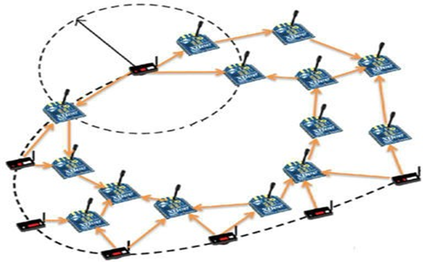
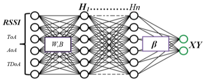
In the last decade, the Machine Learning Techniques (MLT) in WSNs have received a particular attention. Artificial Neural Network (ANN), Support Vector Machine (SVM), Deep Learning (DL) approach models are applied in different fields for classification problem, density estimation or process identification. Indeed, the MLT technique was used in many WSN configurations such as range-based, range-free, isotropic and anisotropic environments (see Figure 1). In the range-based cases, ANN inputs (Figure 2) represent some physical characteristics of the received signals such as the RSSI, ToA, TDoA and/or the AoA [1-4]. These ANN-Range-Based models give good localization performances, but they need extra hardware equipment. In ANN-Range-Free techniques, based on WSN connectivity and anchors positions, location of unknown nodes is estimated without additional devices. The ANN-Range-Free localization model could be used for any type of Isotropic-WSN and gives acceptable accuracy.
(a)
(b)
Figure 1. Isotropic WSN deployment (a: without obstacles) and Anisotropic WSN deployment (b: with obstacles)
Figure 2. Range based Deep-ANN localization modes
In this work, a novel ANN-Range-Free model based on Cascade-ELM algorithms for WSN localization is proposed. Different scenarios in isotropic environments will be considered to experiment the suggested algorithm and to show the efficacy of the proposed technique. The rest of this paper is presented as follows. Section 2 is dedicated to the review of the state of the art on localization problem in WSN. In section 3 and 4 we present respectively the basic single hidden layer ELM and the cascade ELM and their application for the localization task. Section 5 is dedicated to the analysis of simulation results and the comparison of the proposed ELM architectures performances. Finally, the conclusion and future works are given in section 6.
Recently, the WSN localization issue was treated by different research works using Artificial Intelligence (AI) and Machine Learning Techniques (MLT) such as ANN, SVM, ELM (Extreme Learning Machine) and Deep learning [5-7]. In a WSN scenario, identifying the current location of a sensor node is primordial to give more confidence to the collected data. For example, Chang et al. exploit the machine learning ELM to find the appropriate sub-anchor nodes for localization process via the improved DV-Hop localization algorithm. Firstly, the called DV-Hop-ELM upgrades several virtual unknown nodes to sub-anchor nodes via the ELM process. The sub-anchor and real anchor nodes are used together to locate the remaining unknown nodes by the classic DV-Hop algorithm [8, 9]. Peng et al. [10] proposed combination of the Genetic Algorithm metaheuristic and the Dv-Hop algorithm to compute unknown node coordinates in WSNs. In fact, by using the feasible population region defined by the Max-Min techniques, the optimization localization process via the genetic algorithm is applied for minimizing the localization errors. Zhu and Wei [11] presented a fast-SVM for large scale WSNs localization algorithm. The proposed localization algorithm transforms the location estimation position of the WSNs into multiclass problem, and the binary support vector machine for localization is used to solve this issue. The proposed fast-SVM introduces the similarity measure, and the support vectors can be divided into groups according to the maximal similarity measure. Moreover, Zheng et al. used the Regularized ELM-WSN to treat multi-hop localization problem. The suggested algorithm uses the following steps: sensing learning data via the correspondence between the number of hops and the physical distances separating known and unknown nodes, and the Trilateration algorithm for the localization process [12]. Phoemphon et al. presented the hybrid localization models based on fuzzy logic and ELM model. To optimize the localization accuracy, the PSO minimizes the effects of irregular deployments [13].
Javadi uses the Support Vector Machine and its variant Twin-SVM for sources localization in WSN. Javadi considers that the Twin-SVM localizes the area of the expected node position and uses the distributed learning algorithm for this localization process. The average position of the nodes in the sensing area can be considered as the position of the event that needs to be located [14]. Recently, Wang et al. suggested the exploitation of the Kernel Extreme Learning Machines based on hop-count quantization (KELM-HQ) for localization problem in range-free WSNs. The suggested method computes the expected real number of hop-count between anchors and unknown nodes. For the training phase, the inputs and target outputs of the KELM are respectively the hop-count number (between anchors and unknown nodes) and the anchors locations. Using the linear-kernel, the proposed method uses the real quantized hop-counts between unknown nodes as the test samples for the localization process in the exploitation phase [15]. In Liouane et al, the authors proposed a novel approach for localization in WSN based on Machine Learning Technique such as online sequential extreme learning machine (OS-ELM) for multi-hop WSN. The proposed localization algorithm greatly reduces the average localization error in comparison with the original DV- Hop heuristic [16].
In WSN, it has been proved that there exists a direct correlation between minimum hop count and the corresponding physical distance. Extreme Learning Machine model could be used for the localization of unknown nodes in the WSN. In the first learning phase, a beacon’s packet is broadcasted by each anchor node within the sensing network to inform other nodes about anchors information (ID and hop-count values). Once a node received this packet the sensor node increments its hop-count. Then, each node computes its cumulative minimum hops counts between them and the anchor nodes.
3.1 WSN discovery
Like the first step of the basic DV-Hop algorithm is called flooding phase, in the first learning phase, a beacon’s packet is broadcasted by each anchor node within the sensing network to inform other nodes about anchors information (ID and hop-count values). Once a node received this packet the sensor node increments its hop-count. Then, each node computes its cumulative minimum hop-count between them and the anchor nodes. For example, in Figure 1 (a), the hop-count between anchor A1 and the node n5 is given by the min(hc11, hc14)+1 =min(1,3)+1=2. As a result, the minimum’s hop-count between all nodes is given and provides the global hop count matrix HC. The HC matrix is divided into two sub-matrix Hca and Hcn designing the anchors connectivity and the unknown nodes connectivity. Moreover, the anchors connectivity Hca matrix represents reference nodes for the learning phase. When the coordinates Xa of all anchor nodes are known the distances matrix Da of the anchor nodes can be directly calculated.
$H C=\left(\begin{array}{l}{[H c a]} \\ {[H c n]}\end{array}\right) \in R^{(n a+n n) \times n a}, D=\left(\begin{array}{l}{[D a]} \\ {[D n]}\end{array}\right) \in R^{(n a+n n) \times n a} \quad, X Y=\left(\begin{array}{l}{[X a]} \\ {[X n]}\end{array}\right) \in R^{(n a+n n) \times 2}$
3.2 WSN localization learning phase via the ELM model
The 2-dimentionnal WSN is composed by (n) randomly deployed nodes which are divided in two groups respectively (na) anchors nodes and (nn) unknown nodes. The hop-count between all sensor nodes is represented by the HC matrix, the distances between all sensors are given by D matrix and XY matrix represents the locations of all sensor’s nodes.
3.2.1 The first layer of the ELM interpretation
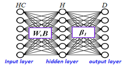
We suppose that the relation between hop-count matrix HC and the distance matrix D can be expressed by the machine learning process via the ELM given by Figure 3.
Figure 3. The first ELM learning phase
The hidden layer matrix can be expressed by:
$H=\left[\begin{array}{ccc}g\left(H C_1 W_1+b_1\right) & \cdots & g\left(H C_1 W_z+b_z\right) \\ \vdots & \ddots & \vdots \\ g\left(H C_{n a+n n} W_1+b_1\right) & \cdots & g\left(H C_{n a+n n} W_z+b_z\right)\end{array}\right]$ (1)
$H=\left(\begin{array}{l}{[g(H c a, W, B)]} \\ {[g(H c n, W, B)]}\end{array}\right)=\left(\begin{array}{l}{[H a]} \\ {[H n]}\end{array}\right)$ (2)
with $H \in R^{(n a+n n) \times z}, \beta_1 \in R^{z \times n a}$ and $D \in R^{(n a+n n) \times n a}$
where, g represents the sigmoid activation function.
According to the ELM theory, the output layer is given by the least square method [17-19].
$H \cdot \beta_1=D \Rightarrow\left(\begin{array}{l}{[H a]} \\ {[H n]}\end{array}\right) \cdot \beta_1=\left(\begin{array}{l}{[D a]} \\ {[D n]}\end{array}\right)$$\Rightarrow\left\{\begin{array}{l}{[H a] \cdot \beta_1=[D a] \Rightarrow \text { learning phase }} \\ {[H n] \cdot \beta_1=[D n] \Rightarrow \text { exploitation phase }}\end{array}\right.$ (3)
where, β1 represents the output weight matrix of the ELM model and can be calculated in the learning phase via the least square optimization method.
$\beta_1=\left(H a^T H a\right)^{-1} H a^T D a$ (4)
where,
$H a=g\left(H C_a, W, B\right)$ (5)
The reduced number of the anchor nodes for the training phase introduces the problem of underfitting or overfitting. Reducing these problems and ameliorating the generalization error of the localization process needs a regularization factor “α” for the output weight β1 estimation. The “α” parameter allow adjusting the weights of the ELM with respect the generalization error in the exploitation phase.
Using the regularized ELM, β1 expression becomes:
$\beta_1=\left(H a^T H a+\alpha I d\right)^{-1} H a^T D a$ (6)
where, Id denotes the (z×z) identity matrix.
3.2.2 The second layer of the ELM interpretation
Moreover, we suppose that the relation between distance matrix D and the coordinates XY of all nodes can be computed by ELM model and can be calculated in the second learning phase via the least square optimization method:
$D \beta_2=X Y \Rightarrow\left(\begin{array}{l}{[D a]} \\ {[D n]}\end{array}\right) \cdot \beta_2=\left(\begin{array}{l}{[X a]} \\ {[X n]}\end{array}\right)$$\Rightarrow \begin{cases}{[D a] \beta_2=[X a]} & \text { learning phase } \\ {[D n] \beta_2=[X n]} & \text { exploitation phase }\end{cases}$ (7)
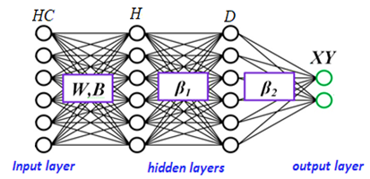
where, β2 Rna×2 represents the output weight matrix of the second hidden layer and can be calculated via the Cascade-ELM. Figure 4 gives the structure of the Cascade-ELM model.
$\beta_2=\left(D a^T D a\right)^{-1} D a^T X a$ (8)
Figure 4. The cascade ELM learning phase
3.3 The WSN localization phase
3.3.1 The distance estimation
Using the previous calculation, the distances between all unknown nodes and anchor nodes are given by:
$D n=H n \beta_1$
$D n=H n\left(H a^T H a\right)^{-1} H a^T D a$ (9)
where,
$H n=g\left(H C_n, W, B\right)$ (10)
3.3.2 The localization process
From the previous calculation as well, the expected positions Xn of all unknown nodes are given by:
$X n=D n \beta_2$
$X n=D n\left(D a^T D a\right)^{-1} D a^T X a$ (11)
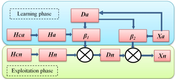
Figure 5 resumes the WSN localization process approximation.
Figure 5. The Cascade ELM model for WSN localization process
In this section we conduct simulation to check the localization accuracy of our Cascade-ELM algorithm in isotropic case with N=300 unknown nodes. The localization errors of the proposed Cascade-ELM algorithm are compared with those of KELM-HQ, the fast-SVM, the GADV-Hop and the DV-Hop-ELM algorithms. These last algorithms, issued from soft computing techniques, are chosen for comparison thanks to their good localization accuracy compared with the improved traditional DV-Hop heuristic. Matlab tools are used for the implementation and the simulations of Cascade-ELM. We conduct 50 times randomly deployment scenarios simulation, and we computed the average values of these simulations. In the first part of simulation, the unknown nodes are deployed in a 2-D sensing field of surface S=100 m×100 m. All nodes have the same communication range R=10 m. The number of anchor nodes is set to 5, 10, 15, 20, 25, 30 and 35. During the localization phase, we assume as well that every node in the network communicates with the others by the multi-hop routing protocol. The first hidden layer uses 200 neurons as well as the sigmoidal activation function. Moreover, during the exploitation step, the weight matrix W and Bias remain the same as those used in the learning step.
We use the average localization error (ALE) to measure the accuracy of our proposed localization schemes.
$A L E=\frac{1}{N \times R} \sum_{i=1}^N \sqrt{\left(x_i^{\text {est }}-x_i\right)^2+\left(y_i^{\text {est }}-y_i\right)^2}$ (12)
where, N=300 and R=10m are the total amount of the unknown nodes and the communication radio, respectively. The (xi, yi) present the real position and the (xest, yest) are estimated position of the i’th unknown node.
4.1 Results and comparison for isotropic WSN
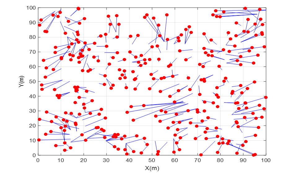
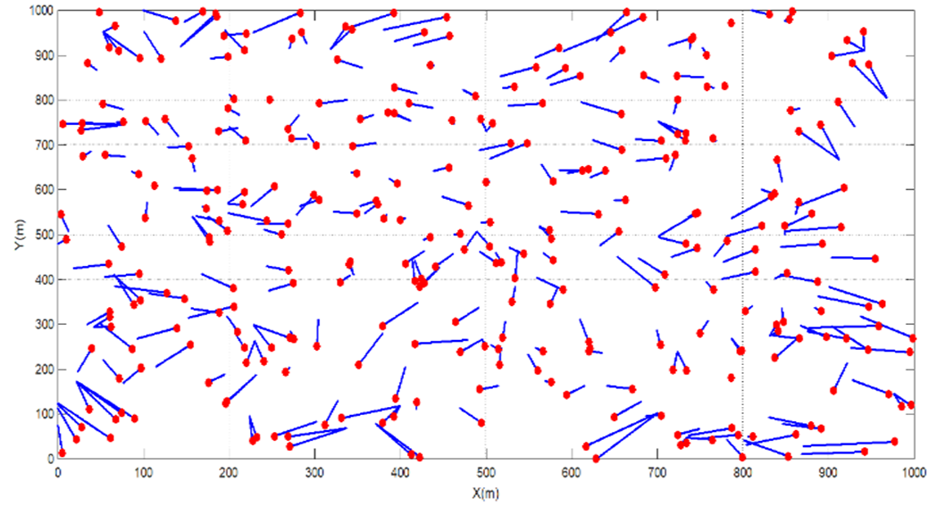
Figures 6 to 9 give an example of localization results using the Cascade-ELM for different anchor deployment scenarios. The deployed environment is made up of 300 sensor nodes and the adopted communication range is of 10 m. The actual position of each unknown node is indicated by the red point and the error between the exact position and the estimated one is represented by the blue line. As seen in these figures and as expected, for the tree localization results, the accuracy of localization is improving as the number of anchor nodes in the network is increasing. In fact, the increase of the number of anchors leads to increase the number of reference nodes then increase the number of information for localization phase.
Figure 6. Localization results for 5 anchors and 300 nodes and R=10m
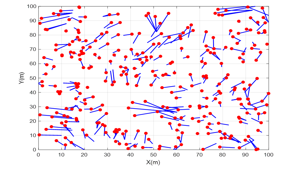
Figure 7. Localization results for 20 anchors and 300 nodes and R=10m
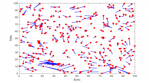
Figure 8. Localization results for 35 anchors and 300 nodes and R=10m
Figure 9. Localization results for 50 anchors and 300 nodes and R=10m
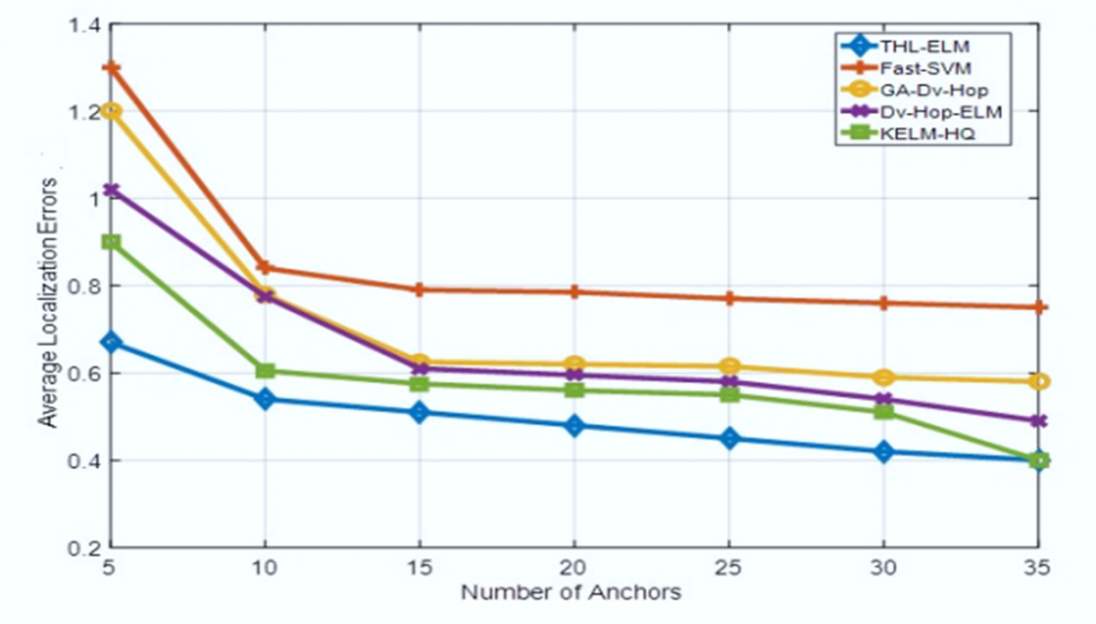
As expected in Figure 10, for the KELM-HQ, the fast-SVM, the GADV-Hop, the DV-Hop-ELM and the Cascade-ELM algorithms, increasing the number of anchor nodes improves the accuracy of locating nodes. In fact, the increase of the number of anchors leads to increase the number of references
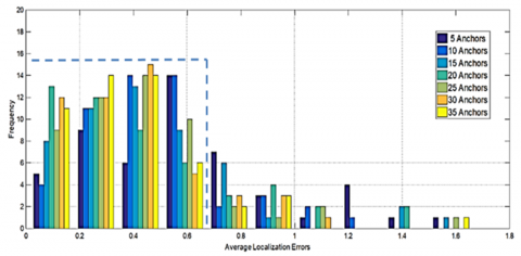
nodes, and by the way improves the information for the training phase. Furthermore, the localization error of the proposed Cascade-ELM algorithm was largely smaller than that of its counterparts. In fact, the proposed Cascade-ELM algorithm accuracy increased over 5%, 25%, 15%, and 10% when compared with KELM-HQ, fast-SVM, GADV-Hop and the DV-Hop-ELM, respectively. Therefore, boosted by the first layer for real distance estimation between anchors and unknown nodes our Cascade-ELM algorithm outperforms in terms of localization accuracy in comparison with the other four algorithms. Consequently, the expected distance between anchors and unknown node corresponds more to the real distance. Hence, the average positioning error will decrease. Figure 11 and Table 1 show the histogram of repartition errors and the statistical results of localization error with different number of anchors. The results are for 50 random simulation runs. It is noted that in the majority of the cases of simulation we obtain an error of localization lower than 0.6×R.
Figure 10. Localization error of the KELM-HQ, the fast-SVM, the GADV-Hop, the DV-Hop-ELM and the Cascade-ELM algorithms for 5.35 anchors and 300 unknown nodes and the communication range of each node is R=10m
Table 1. Performance results of the Cascade-ELM localization process
|
|
5 |
10 |
15 |
20 |
25 |
30 |
35 |
|
Min |
0.27 |
0.21 |
0.23 |
0.20 |
0.24 |
0.20 |
0.20 |
|
Max |
1.65 |
1.61 |
1.56 |
1.45 |
1.3 |
0.97 |
0.96 |
|
Mean |
0.69 |
0.53 |
0.51 |
0.48 |
0.45 |
0.42 |
0.40 |
|
Std |
0.44 |
0.38 |
0.21 |
0.31 |
0.24 |
0.30 |
0.28 |
Figure 11. Histogram of the ALE for 50 simulation runs
4.2 Degree if irregularity signal effects
Practically, in sensor networks the sensed environment is affected by many irregularity effects like the electromagnetic noise and the RSSI variation, thus the radio communication of the RF sensor nodes will take the form of an irregular elliptic form instead of a standard circle [20, 21]. The impact of radio irregularity on routing protocol can affect the minimum hop counts for localization process in range free WSN. Many researches investigate the characterization of degree of radio irregularity signal. Indeed, the degree of irregularity (DOI) model draws the maximal variation of radio range per unit degree change within different directions of radio propagation antenna.
In the following simulation phase, we exploit the most used DOI model to study the impact of communication irregularity phenomena. In fact, the probability that two nodes can communicate with each other is controlled by a parameter (d). The next model describes the connectivity probability for two nodes separated by the distance (d) and the ideal communication range R. In this model the probability of the connectivity is described by:
$P_d= \begin{cases}1 & \frac{d}{\mathrm{R}}<1-\mathrm{DOI}, \\ \frac{1}{2 \times \mathrm{DOI}}\left(\frac{d}{\mathrm{R}}-1\right)+\frac{1}{2}, & 1-\mathrm{DOI} \leq \frac{d}{\mathrm{R}} \leq 1+\mathrm{DOI} \\ 0, & \frac{d}{R}>1+\mathrm{DOI}\end{cases}$ (13)
As shown in Figure 12, the transmission radio changes with the value of DOI. When DOI = 0, the transmission radio R takes the form of an ideal circle. Moreover, as the value of DOI increases as the irregularity of the transmission range increases and affects the number of hops between anchor nodes and the localized nodes. In our simulation, the DOI signal permits to represent the propagation irregularities in WSN localization process.
Figure 12. DOI effects on the irregularity radio communication
To study the DOI effect on the Cascade-ELM localization process and find the correlation between localization errors and the DOI, we implement the localization algorithm with the model of radio range irregularity, and we suppose that sensor nodes have the same transmission range of radius R=100m. DOI is varied between [0,0.07]. In the simulation cases, 300 unknown nodes are deployed in a 2-D area of a surface S=1,000m×1,000m with the average communication range R=100m and the number of anchor nodes is equal to 50.
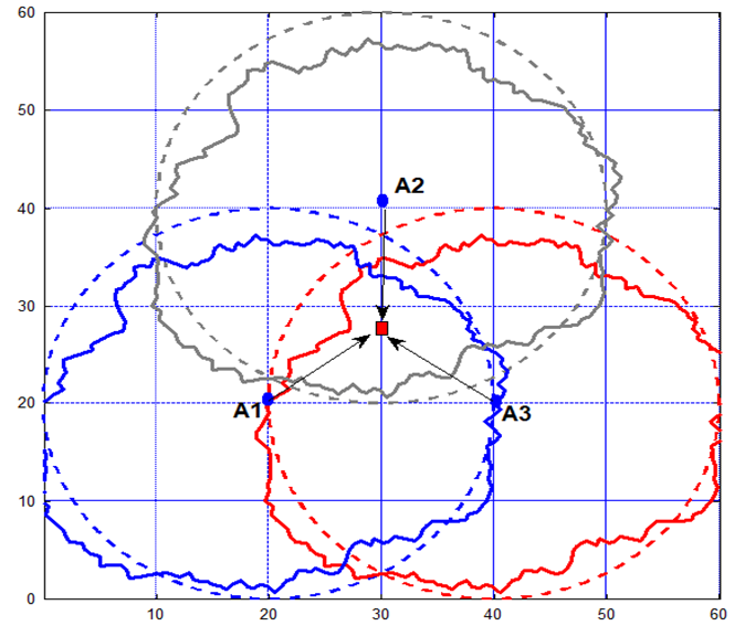
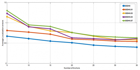
Figure 13 gives the simulation results of the ALE for different anchors deployment and for different values of the DOI. As seen in this figure, when the number of anchor is reduced, it is clear that with the increase of DOI the LE is greater than the communication range R. This statement is expected because when the DOI increases, the connectivity of the network is perturbed, thus the ALE will increases. Figure 14 shows an example of localization results given by the proposed Cascade-ELM localization process.
Figure 13. The localization errors for different DOI values
Figure 14. Sample simulation run for deployment zone 1,000 × 1,000 m², 50 anchors, 300 unknown nodes and the average communication range of each node is R=100m
As expected, if the DOI increases then the connectivity of the wireless sensors network is perturbed and the hop counts between anchors and unknown nodes is affected, then the localization accuracy will be deteriorated. For example, for 35 anchor nodes, if the DOI is 0 then the ALE is near to 0.4 × R but if the DOI=0.07 the ALE is near to 0.7 × R because the hop count value is affected and introduces ALE. Moreover, for 5 anchor nodes, if the DOI is 0 then the ALE is near to 0.75 × R but if the DOI=0.07 the ALE is near to 1.35 × R because the hop count value is largely affected and introduces a large localization error.
In this work, a deep neural network algorithm based on the cascade ELM has been suggested in order to improve the node localization performance in WSN. The proposed cascade ELM algorithms are based on range free technique in isotropic cases. The cascade-ELM represents a new way to tackle the WSN localization problem. They have been experimented via simulation for many scenarios in isotropic environments. The average localization errors have been applied to evaluate the performance of the localization model. The performance of the proposed localization algorithms is well shown through simulation results when compared with the other soft-computing algorithms in term of ALE. Boosted by the expected first layer of the ELM for hop-size estimation and the second layer for the positions estimation, the experimental results demonstrate that the Cascade-ELM localization algorithm for localization in WSNs minimizes the average localization error of nodes and has higher location accuracy compared with its counterparts.
[1] Hatami, A., Pahlavan, K., Heidari, M., Akgul, F. (2006). On RSS and TOA based indoor geolocation-a comparative performance evaluation. In IEEE Wireless Communications and Networking Conference, 2006. WCNC 2006, Las Vegas, NV, USA, pp. 2267-2272. https://doi.org/10.1109/WCNC.2006.1696648
[2] Wei, X., Wang, L., Wan, J. (2006). A new localization technique based on network TDOA information. In 2006 6th International Conference on ITS Telecommunications, Chengdu, China, pp. 127-130. https://doi.org/10.1109/ITST.2006.288796
[3] Guvenc, I., Sahinoglu, Z. (2005). Threshold-based TOA estimation for impulse radio UWB systems. In 2005 IEEE International Conference on Ultra-Wideband, Zurich, Switzerland, pp. 420-425. https://doi.org/10.1109/ICU.2005.1570024
[4] Femmam, S., Benakila, I.M. (2016). A new topology time division beacon construction approach for IEEE802. 15.4/ZigBee cluster-tree wireless sensor networks. In 2016 IEEE 14th Intl Conf on Dependable, Autonomic and Secure Computing, 14th Intl Conf on Pervasive Intelligence and Computing, 2nd Intl Conf on Big Data Intelligence and Computing and Cyber Science and Technology Congress (DASC/PiCom/DataCom/CyberSciTech), pp. 856-860. https://doi.org/10.1109/DASC-PICom-DataCom-CyberSciTec.2016.146
[5] Sun, G., Guo, W. (2005). Robust mobile geo-location algorithm based on LS-SVM. IEEE Transactions on vehicular technology, 54(3): 1037-1041. https://doi.org/10.1109/TVT.2005.844676
[6] Wang, J., Zhang, X., Gao, Q., Yue, H., Wang, H. (2016). Device-free wireless localization and activity recognition: A deep learning approach. IEEE Transactions on Vehicular Technology, 66(7): 6258-6267. https://doi.org/10.1109/TVT.2016.2635161
[7] Cottone, P., Gaglio, S., Re, G.L., Ortolani, M. (2016). A machine learning approach for user localization exploiting connectivity data. Engineering Applications of Artificial Intelligence, 50: 125-134. https://doi.org/10.1016/j.engappai.2015.12.015
[8] Niculescu, D., Nath, B. (2003). DV based positioning in ad hoc networks. Telecommunication Systems, 22(1): 267-280. https://doi.org/10.1023/A:1023403323460
[9] Chang, X., Luo, X. (2014). An improved self-localization algorithm for Ad hoc network based on extreme learning machine. In Proceeding of the 11th World Congress on Intelligent Control and Automation, Shenyang, China, pp. 564-569. https://doi.org/10.1109/WCICA.2014.7052775
[10] Peng, B., Li, L. (2015). An improved localization algorithm based on genetic algorithm in wireless sensor networks. Cognitive Neurodynamics, 9(2): 249-256. https://doi.org/10.1007/s11571-014-9324-y
[11] Zhu, F., Wei, J. (2017). Localization algorithm for large scale wireless sensor networks based on fast-SVM. Wireless Personal Communications, 95(3): 1859-1875. https://doi.org/10.1007/s11277-016-3665-2
[12] Zheng, W., Yan, X., Zhao, W., Qian, C. (2017). A large-scale multi-hop localization algorithm based on regularized extreme learning for wireless networks. Sensors, 17(12): 2959. https://doi.org/10.3390/s17122959
[13] Phoemphon, S., So-In, C., Niyato, D.T. (2018). A hybrid model using fuzzy logic and an extreme learning machine with vector particle swarm optimization for wireless sensor network localization. Applied Soft Computing, 65: 101-120. https://doi.org/10.1016/j.asoc.2018.01.004
[14] Javadi, S.H., Moosaei, H., Ciuonzo, D. (2019). Learning wireless sensor networks for source localization. Sensors, 19(3): 635. https://doi.org/10.3390/s19030635
[15] Wang, L., Er, M.J., Zhang, S. (2020). A kernel extreme learning machines algorithm for node localization in wireless sensor networks. IEEE Communications Letters, 24(7): 1433-1436. https://doi.org/10.1109/LCOMM.2020.2986676
[16] Liouane, O., Femmam, S., Bakir, T., Abdelali, A.B. (2021). On-line Sequential ELM based localization process for large scale Wireless Sensors Network. In 2021 International Conference on Control, Automation and Diagnosis (ICCAD), Grenoble, France, pp. 1-6. https://doi.org/10.1109/ICCAD52417.2021.9638725
[17] Huang, G.B., Liang, N.Y., Rong, H.J., Saratchandran, P., Sundararajan, N. (2005). On-line sequential extreme learning machine. Computational Intelligence, 2005: 232-237.
[18] Huang, G.B., Wang, D.H., Lan, Y. (2011). Extreme learning machines: A survey. International Journal of Machine Learning and Cybernetics, 2(2): 107-122. https://doi.org/10.1007/s13042-011-0019-y
[19] Huang, G.B., Zhu, Q.Y., Siew, C.K. (2006). Extreme learning machine: theory and applications. Neurocomputing, 70(1-3): 489-501. https://doi.org/10.1016/j.neucom.2005.12.126
[20] Xiao, Q., Xiao, B., Cao, J., Wang, J. (2010). Multihop range-free localization in anisotropic wireless sensor networks: A pattern-driven scheme. IEEE Transactions on Mobile Computing, 9(11): 1592-1607. https://doi.org/10.1109/TMC.2010.129
[21] Laoudias, C., Moreira, A., Kim, S., Lee, S., Wirola, L., Fischione, C. (2018). A survey of enabling technologies for network localization, tracking, and navigation. In IEEE Communications Surveys & Tutorials, 20(4): 3607-3644. https://doi.org/10.1109/COMST.2018.2855063