Abderrahmane El Mettiti* | Mohammed Oumsis
© 2022 IIETA. This article is published by IIETA and is licensed under the CC BY 4.0 license (http://creativecommons.org/licenses/by/4.0/).
OPEN ACCESS
The millimeter-wave frequencies planned for 6G systems present challenges for channel modeling. At these frequencies, surface roughness affects wave propagation and causes severe attenuation of millimeter-wave (mmWave) signals. In general, beamforming techniques compensate for this problem. Analog beamforming has some major advantages over its counterpart, digital beamforming, because it uses low-cost phase shifters for massive MIMO systems compared to digital beamforming that provides more accurate and faster results in determining user signals. However, digital beamforming suffers from high complexity and expensive design, making it unsuitable for mmWave systems. The techniques proposed so far for analog beamforming are often challenging in practice. In this work, we have proposed a deep learning model for analog beams training that helps predict the optimal beam vector. Our model uses an available dataset of 18 base stations, over 1 million users, 60 GHz frequency. The training process first applies a stacked autoencoder to extract the features from the training datasets, and then uses a multilayer perceptron (MLP) to train and predict the optimal beams. Then, the results are evaluated by computing the mean squared error between the expected and predicted beams using the test set. The results show high efficiency compared to the benchmark method, which uses only the MLP for the training process.
6G networks, beamforming, artificial intelligence, deep learning, autoencoders, millimeter-wave
The standardization of fifth-generation services has created fierce competition to develop new-generation services on a global scale. The United States, Japan, South Korea and other developed countries, as well as some European countries, have begun to study and formulate the development plan for sixth-generation technology [1].
6G technology will realize data-driven and machine learning-based systems that integrate artificial intelligence (AI) technologies. These new communication architectures are designed to realize comprehensive self-organization, self-learning, self-healing, self-aggregation, self-protection, and self-optimization of the network.
Artificial intelligence (AI) will also help 6G deliver highly personalized and connected intelligent services to individuals, businesses and other users to meet refined needs [2, 3].
Although the specifications of 6G, such as frequency bands and data rate requirements, have not yet been finally defined, its applications have already been considered. A consensus has been reached for 6G - 6G will be an intelligent mobile communications network of much larger scale that encompasses 5G [4, 5]. While the quasi-two-dimensional 5G network covers only a limited portion of the globe, the 6G network will extend in three dimensions, connecting satellites, aircraft, ships, and land-based infrastructures and providing truly global coverage. The mmWave technologies will play an important role in enabling the various wireless connections with higher speed and reliability than 5G. In addition, the use of terahertz as part of the frequency bands for 6G communications has also been proposed [5]. However, the corresponding key devices of terahertz chips, front-end components, and systems are not yet as mature and reliable as those operating at mmWave frequencies for long-range, high-fidelity communications. Millimeter-wave communications can fully exploit the abundant spectrum resources in the frequency band above 26 GHz to realize ultra-high-speed data transmissions and 0.1−10 THz band expected for the 6G era [6]. At the same time, the higher the working frequency band of millimeter-wave communications, the greater the scattering loss. Researchers often use large antenna arrays to form multiple-input multiple-output (MIMO) systems to generate highly directional beams and compensate for scattering loss.
In addition, 6G is supported by an unexpected speed level that can reach 1 TB per second [7]. This will improve the performance of 5G applications and increase its ability to support new and innovative applications. To achieve this speed, 6G should include the use of very high frequencies (millimeter waves) of the radio spectrum. The bandwidth capacity of the 5G network is due to the use of high radio frequencies; the higher the radio spectrum, the more data can be transmitted. The sixth-generation (6G) network could eventually approach the upper limit of the radio spectrum, reaching very high frequencies in the 300 GHz or even terahertz bands [2, 8-11].
For these reasons, several methods and approaches for millimeter-wave beam selection have been proposed. Beam selection uses simulated transmit and receive beams to detect millimeter-wave MIMO channels and find the combination of receive and transmit beams with the largest received signal energy, i.e., the most suitable beam pair for channel transmission, avoiding the need for large-dimensional air interfaces data.
Inspired by the great breakthroughs achieved by deep learning (DL) in computer vision and natural language processing, DL has also been used for wireless communication [12]. Compared to methods based on mathematical models, DL offers two key advantages. First, mathematical tools are generally based on idealized assumptions, such as the presence of pure additive white Gaussian noise, which may not be compatible with practical scenarios. In contrast, DL adaptively learns the characteristics of the channel to support reliable beam training [13]. Second, the parameters of the DL models capture the high-dimensional features of the propagation scenario. For these reasons, this paper investigates DL techniques for training beams since they are very well suited to deal with the nonlinear and nonmonotonic properties of channel power leaks in mmWave communications. The paper is organized as follows: Section 2 presents the previous works of mmWave beamforming, Section 3 describes the beamforming training problem, the dataset used and the deep learning algorithms studied, Section 4 explains our proposed approach, Section 5 evaluates and discusses the results, and finally Section 6 summarizes the goal of our work and perspectives.
Millimeter waves are the critical components of wireless communication systems, posing challenges in training and selecting the best beam. Several previous works focused on selecting the optimal mm-wave beam using machine learning and deep learning techniques. Wang et al. proposed a machine learning approach combined with situation awareness for beam training. They considered observations of the vehicle environment, receiver locations, and surrounding vehicles [14]. The authors used multimodal neural networks to learn the beams using a dataset from the wireless communication environment. In addition, they evaluated their approach on a real vehicle dataset [15]. They used image classification and residual networks to predict beam and blockage directly from RVB cameras and sub-6 GHz channels [16]. Tarun et al. [17] proposed a deep neural network model for millimeter-wave beam prediction by mapping the complex patterns from received signal strengths to the receiver's optimal spatial beam. The authors focused on a small number of beams to detect the best beam faster. Alrabeiah et al. [18] realized an advanced dataset with different base stations, mobile users, and rich dynamics. They also proposed visual wireless mm-wave beam tracking with recurrent neural networks. Bian et al. [19] implemented a two-input neural network, which they named fusionNet, to predict the best mm-wave beam. They proposed to use channel sparsity and data augmentation to avoid the overfitting problem. Ma et al. used the low-frequency channel state information to extract out-of-band information and predict the mm-wave beam with deep learning [20]. Catak et al. [21] proposed an artificial neural network to predict mm-wave beams using a realistic dataset and then applied an adversarial machine learning method to increase the prediction security. Alrabieh et al. [22] proposed learning mapping functions and predicting the optimal beam and blockages directly from the sub-6 GHz channel. Ying et al. [23] used object recognition to locate users based on the RGB images captured by the cameras. Then they used a multilayer perceptron to predict the angles between the users and the cameras. They then selected the optimal beam according to the extracted angle information and a predefined beam codebook. Aldalbahi et al. [24] investigated long-term memory for instantaneous prediction of alternative beam directions when the main beam is blocked. In the same context, this work focused on predicting the optimal beam using a simple and a real-time solution to increase the reliability and accuracy of mmWave systems for the sixth generation of mobile applications without consuming a high cost and time. In our strategy, the serving base station uses the beam sequence it has offered to mobile users in the past to predict the best beams for the following instants. This enables improved system reliability and reduced latency overhead. To this end, we develop a deep learning model based on multilayer perceptrons and a stacked autoencoder for feature extraction. Simulation results show that the proposed solution predicts the optimal beams with minimal error, improving the reliability of the mmWave large antenna system.
3.1 mmWave beamforming prediction
6G mobile networks are a key enabler for transmitting large amounts of data with low latency. However, with the deployment of more bandwidth, 6G networks also face the problem of high path loss in the MMwave band. To address this degradation, beamforming technology has been applied to improve antenna gain by establishing a highly directional transmission link between user equipment (UE) and mmWave node base stations (gNBs).
Beamforming is a spatial filtering technique that uses an array of radiators to capture or radiate energy in a specific direction of an aperture. An improvement over omnidirectional transmit/receive is transmit/receive gain. In modern communication systems, smart antenna systems are used to combine array gain with diversity gain while suppressing interference and increasing the capacity of the communication link. This is achieved by using a phased array and a radiation setup consisting of several elements with a specific geometric configuration to control the electronic beam.
Beamforming is an important requirement for 6G networks, which operate in the mmWave frequency band to improve network coverage. Depending on the unit that performs the signal processing, i.e. in the baseband or RF range, beamforming is classified into digital beamforming (DBF), analog beamforming (ABF), and hybrid beamforming (HBF) [25].
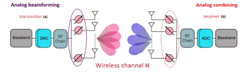
In this paper we study the ABF. In ABF, a single signal is delivered via analog phase shifters to each antenna element in the array, where the signal is amplified and radiated to the desired receiver. Amplitude/phase variation is applied to the analog signal at the end of the transmission, adding the signals from the different antennas before analog-to-digital conversion. Analog beamforming is the most economical way to build a beamforming network, but it can only manage and generate one signal beam. Figure 1 shows the architecture of the analog beamforming; Analog beamforming is realized by a phased array with only a radio frequency chain controlled by a digital-to-analog converter in the transmitter or an analog-to-digital converter in the receiver. A transmitter RF chain consists of a frequency up-converter, a power amplifier, etc.; a receiver RF chain consists of a low-noise amplifier, a frequency down-converter, etc.
Figure 1. Receiver and transmitter analog beamforming architecture (RF: Radio frequency, DAC: digital-to-analog converters, ADC: analog-to-digital converter)
Figure 1(a) illustrates an analog beamforming transmitter: the transmitted baseband signal is first modulated. This radio signal is divided with a power divider and passes through the beamformer, which can change the amplitude (ak) and phase shift (θk) of the signals in each of the paths leading to an antenna stack. The power divider depends on the number of antennas used in the antenna stack.
Figure 1(b) illustrates an analog beamforming receiver. As the block diagram of the receiver shows, complex weighting is applied to the signal from each antenna in the array. The complex weighting includes both amplitude and phase shift (Formula 1 and 2). Then the signals are combined to produce an output signal, which provides the desired directional pattern of an antenna array [25].
$W_{k}=a_{k} * e^{j \sin (\theta)}$ (1)
$W_{k}=a_{k} * \cos (\theta k)+j a_{k} \sin (\theta k)$ (2)
where, Wk is the complex weights of the K-th network antenna, ak is the relative amplitude of weights, and Ɵk is the phase shift.
In mmWave communications, large-scale antenna arrays are used to generate highly directional beams to compensate for severe path loss. Beam prediction avoids estimating high-dimensional channel matrices by selecting the best beam. Leveraging machine learning algorithms is a novel solution for mmWave training and scanning of a large number of narrow beams. Beams depend on environmental conditions such as user location and base station location, furniture, trees, buildings, etc. It is difficult to define these environmental conditions in closed-form equations. The solution is to use omnidirectional and quasi-omnidirectional beam patterns to predict the optimal RF beamforming vector. The advantage of using these beam patterns is that reflections and diffractions of the pilot signal can be taken into account.
A deep learning solution consists of two phases: training and prediction. First, the deep learning model learns the beam based on the received omnidirectional pilots. Second, the model uses the trained data to predict the current state of the RF beamforming vector. The following sections present the principal aspects of our suggested beamforming prediction approach.
3.2 Dataset presentation
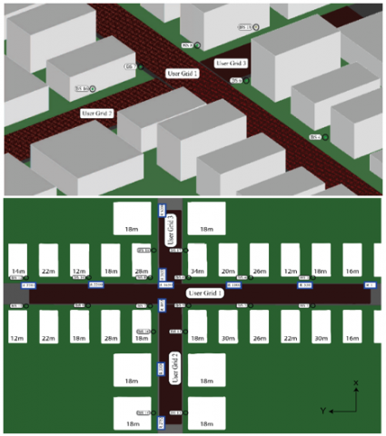
In this work, we used the DeepMIMO dataset generator for mmWave applications presented in ref. [26], applying the O1 scenario. Figure 2 illustrates the bird's eye view and the top view of the O1 ray-tracing scenario, which represents an outdoor area with two streets and one intersection, with 18 BS and more than one million users and 60 GHz frequency. To generate this dataset, we have considered the following parameters:
The active base stations: 3, 4,5, and 6.
The active users: 1000-1300.
The number of BS antenna: Mx=1, My=32, Mz=8.
Antenna spacing: 0.5.
Number of OFDM subcarriers: 1024.
OFDM sampling factor: 1.
OFDM limit: 64.
Number of paths: 5.
Figure 2. Bird’s eye view and top view of the scenario O1 [26]
3.3 Deep learning studied model
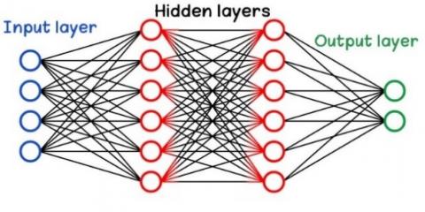
Artificial Neural Networks (ANNs) are biologically inspired computer networks. Among the different types of artificial neural networks, this article focuses on Multilayer Perceptrons (MLPs) with back-propagation learning algorithms. MLPs are commonly used to solve various problems, are complementary to feedforward neural networks. It consists of three types of layers - the input layer, the output layer, and the hidden layer, as shown in Figure 3. The input layer receives the input features to be processed. Required tasks such as prediction and classification are performed by the output layer. An arbitrary number of hidden layers located between the input and output layers is the actual computational engine of MLP. Similar to feedforward networks, data in MLP flows from the input layer to the output layer in the forward direction. The neurons in an MLP are trained using a backpropagation learning algorithm. MLP is designed to approximate any continuous function and can solve linearly inseparable problems. The main use cases for MLP are pattern recognition, classification, prediction and approximation [27].
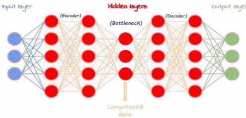
An autoencoder is a special type of ANNs that condenses inputs into a low-dimensional code and rebuilds the output from this representation. The code is the compression of the inputs. An autoencoder is composed of three main components: Encoder, Code, and Decoder. The encoder compresses the input and generates a code. The decoder then uses only this code to reconstruct the output.
Figure 4 depicts the architecture of the autoencoder. Firstly, the input goes through the encoder, which is a fully connected artificial neural network, to generate the code (bottleneck). The decoder has a similar ANN design but uses only the code to generate the output. The goal is to get the same output as the input. Note that the architecture of the decoder is the corresponding image of the encoder. This is not required but is usually the case. The only condition is that the dimensions of the input and the output must be the same. Anything in between can be played.
Figure 3. Multilayer perceptrons architecture
Figure 4. The autoencoder architecture
The mmWave channels data is nonlinear and has a complex nature.
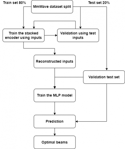
Figure 5. Our proposed beam training using a stacked autoencoder and multilayer perceptrons
For the prediction of mmWave channels, we propose to use a stacked autoencoder to extract the features from the dataset and an MLP model to predict the optimal beams. Figure 5 depicts the architecture of our proposed model, which we construct by following a number of steps namely the data acquisition and preprocessing, feature extraction, and training process.
4.1 Dataset acquisition and generation
In this step, we use the dataset described in section 3.2. To create the framework of the DeepMIMO dataset shown in Figure 2, we defined the ray tracing scenario and parameters to generate the dataset adopted for our application. Specifically, the steps to create this dataset can be summarized as follows:
To prepare the dataset for the following steps, we divided it into two subsets: the training set, which contains 80% of the global data, and the test set, which contains the remaining 20%. It is used to evaluate the prediction accuracy.
4.2 Feature extraction
This step consists of extracting the relevant features and characteristics from the data. The relevance of the selected information is estimated based on its ability to influence the prediction. Stacked autoencoders have gained immense popularity due to their amazing success in a variety of areas such as image classification [29] and speech processing [30]. They are automated feature extraction techniques that require little insight into the problem.
Recently, several works [30, 31] have motivated the use of deep networks to effectively learn abstract features in a hierarchical manner. These deep architectures have been shown to provide a more robust and comprehensive representation [31] of the input data.
In this work, we used a stacked autoencoder to extract the important information and reconstruct a simple input representation from the original dataset. The stacked encoder starts by training the original inputs, then we use the model from the beginning to the bottleneck (code part) and ignore its reconstruction part. This proportion of code gives a compressed representation of the inputs.
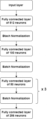
Figure 6 illustrates the autoencoder architecture that we use for the feature extraction. It is composed by multiple fully connected neural layers separated by batch normalization layers. The batch normalization stabilizes the learning process and greatly decreases the number of training epochs needed to train deep neural networks.
Figure 6. The stacked architecture of the proposed autoencoder
4.3 Training process
After reconstructing the input data, we start the training process by applying an MLP model. MLP is often recommended for classification and regression problems. Unlike traditional artificial neural networks, MLP can have many layers of neurons and is capable of learning more complex patterns. It is very flexible and can be used in general to learn a mapping from inputs to outputs. This flexibility allows it to be applied to many types of data such as images, time-series data signals [32, 33], etc. To this end, in our work, we applied an MLP model that uses the uplink pilot received with Omni antennas at multiple base stations to predict the best beamforming vector at each of the coordinating base stations.
MLP is characterised by a high number of hyperparameters. The choice of these values affects the behaviour of the algorithms in terms of error tolerance, variants, number of iterations, etc.
Table 1 shows the optimal hyperparameter values that we adopted after tuning several combinations of our MLP model. We used five hidden MLP layers with a rectified linear unit activation function (reLu) and one output layer with a linear activation function. The reLu function is more powerful than other activation functions because it avoids the problem of the gradient vanishing, which allows the model to learn faster [34]. We also used the Adam optimizer because it can handle noisy problems and is suitable for most problems [35]. After training our model with these parameters, we obtain the beam predictions, which we will evaluate using the test set and the performance metric presented in the next section.
Table 1. The hyperparameters variables used for the MLP model
|
Hyperparameter |
Values |
|
MLP layers (number of units) + Activation function |
1 input layer A hidden layer of 200 units + reLu A hidden layer of 300 units + reLu A hidden layer of 300 units + reLu A hidden layer of 300 units + reLu A hidden layer of 200 units + reLu 1 output layer of 256 unit + linear |
|
Batch size |
128 |
|
Epochs |
20 |
|
Optimizer |
Adam |
|
Loss function |
Mean squared error |
It is important to get the most accurate answers. Claiming wrong results can lead to great losses. To this perspective, this section presents the results of our autoencoder MLP model. The results are evaluated using the mean squared error metric, which we present in the first subsection, and the results are discussed and compared in the second subsection.
5.1 Performance metric
To evaluate the performance of a model the deviation between the predicted values and actual observations is calculated using different statistical methods [36]. In our work, we use Mean Squared Error (MSE), a commonly used and very simple performance metric. MSE represents the squared difference between the actual value and the predicted value. It represents the squared distance between the predicted value and the actual value. This metric is used to avoid the cancellation of negative terms, which is the advantage of MSE. The MSE is calculated according to the formula 3.
$M S E=\frac{1}{N} \sum(y-\hat{y})^{2}$ (3)
where, N is the number of samples; y is the real values and $\hat{y}$ is the predicted values.
5.2 Results discussion
One of the open issues in beamforming prediction research is the difficulty of comparing the performance of papers in the literature due to the diversity of datasets studied and the performance metrics used by the authors. For this reason, we use a simple MLP as a benchmark and compare it with our proposed model.
Figure 7 (a) shows the fitting history of the beamforming prediction with MLP only and Figure 7 (b) shows the fitting history when using MLP and Autoencoders for feature extraction. We can note that the fitting curve of our proposed model is very well fitted compared to the MLP model. This confirms that our model experiences from neither overfitting nor underfitting.
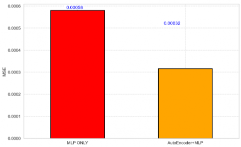
Figure 8 shows the mean squared results of the predicted beams when using MLP only and when using autoencoder for feature extraction and MLP for training. We find that MLP has an error of 0.00058 and our model has an error of 0.00032. This shows the efficiency of the autoencoder for feature extraction because this new set of features summarizes much relevant information contained in the original dataset, which helps to increase the explain ability of the model and speed up model training.
(a)
(b)
Figure 7. (a) The fitting history of the MLP; (b) The fitting history of the stacked autoencoder (for feature extraction + MLP)
Figure 8. The mean squared error of our proposed model against the MLP model only
This article proposes a deep-learning technique for mm-wave analog beamforming prediction. In contrast to the practically challenging existing approaches, our work is very simple and not expensive. It is based on the application of a stacked autoencoder to compress the datasets and Multilayer Perceptrons to train and predict the best beams. Our approach is tested on an available dataset and evaluated using the mean squared error metric. The results were promising and outperformed the benchmark method. For future work, we plan to use different attention-based Deep Learning models and test them in different scenarios of datasets and frequencies.
[1] Dang, S., Amin, O., Shihada, B., Alouini, M.S. (2020). What should 6G be? Nature Electronics, 3(1): 20-29. https://doi.org/10.1038/s41928-019-0355-6
[2] Akhtar, M.W., Hassan, S.A., Ghaffar, R., Jung, H., Garg, S., Hossain, M.S. (2020). The shift to 6G communications: vision and requirements. Human-Centric Computing and Information Sciences, 10(1): 1-27. https://doi.org/10.1186/S13673-020-00258-2
[3] Letaief, K.B., Chen, W., Shi, Y.M., Zhang, J., Zhang, Y.J. (2019). The roadmap to 6G -- AI empowered wireless networks. IEEE Communications Magazine, 57(8): 84-90. https://doi.org/110.1109/MCOM.2019.1900271
[4] Saad, W., Bennis, M., Chen, M. (2019). A vision of 6G wireless systems: Applications, trends, technologies, and open research problems. IEEE Network, 34(3): 134-142. https://doi.org/10.1109/MNET.001.1900287
[5] Rappaport, T.S., Xing, Y., Kanhere, O., et al. (2019). Wireless communications and applications above 100 GHz: Opportunities and challenges for 6G and beyond. IEEE Access, 7: 78729-78757. https://doi.org/10.1109/ACCESS.2019.2921522
[6] Tripathi, S., Sabu, N.V., Gupta, A.K., Dhillon, H.S. (2021). Millimeter-wave and terahertz spectrum for 6G wireless. In 6G Mobile Wireless Networks, pp. 83-121. https://doi.org/10.1007/978-3-030-72777-2_6
[7] Alsharif, M.H., Kelechi, A.H., Albreem, M.A., Chaudhry, S.A., Zia, M.S., Kim, S. (2020). Sixth generation (6G) wireless networks: Vision, research activities, challenges and potential solutions. Symmetry, 12(4): 676. https://doi.org/10.3390/SYM12040676
[8] Khan, L.U., Yaqoob, I., Imran, M., Han, Z., Hong, C.S. (2020). 6G wireless systems: A vision, architectural elements, and future directions. IEEE Access, 8: 147029-147044. https://doi.org/10.1109/ACCESS.2020.3015289
[9] You, X., Wang, C.X., Huang, J., et al. (2021). Towards 6G wireless communication networks: Vision, enabling technologies, and new paradigm shifts. Science China Information Sciences, 64(1): 1-74. https://doi.org/10.1007/S11432-020-2955-6
[10] Tataria, H., Shafi, M., Molisch, A.F., Dohler, M., Sjöland, H., Tufvesson, F. (2021). 6G wireless systems: Vision, requirements, challenges, insights, and opportunities. Proceedings of the IEEE, 109(7): 1166-1199. https://arxiv.org/abs/2008.03213v2
[11] El Mettiti, A., Oumsis, M. (2022). A survey on 6G networks: Vision, requirements, architecture, technologies and challenges. Ingénierie des Systèmes d’Information, 27(1): 1-10. https://doi.org/10.18280/isi.270101
[12] Dai, L., Jiao, R., Adachi, F., Poor, H.V., Hanzo, L. (2020). Deep learning for wireless communications: An emerging interdisciplinary paradigm. IEEE Wireless Communications, 27(4): 133-139. https://doi.org/10.1109/MWC.001.1900491
[13] Qi, C., Wang, Y., Li, G.Y. (2020). Deep learning for beam training in millimeter wave massive MIMO systems. IEEE Transactions on Wireless Communications, 1. https://doi.org/10.1109/TWC.2020.3024279
[14] Wang, Y., Narasimha, M., Heath, R.W. (2018). mmWave beam prediction with situational awareness: A machine learning approach. In 2018 IEEE 19th International Workshop on Signal Processing Advances in Wireless Communications (SPAWC), pp. 1-5. https://doi.org/10.1109/SPAWC.2018.8445969
[15] Charan, G., Osman, T., Hredzak, A., Thawdar, N., Alkhateeb, A. (2021). Vision-position multi-modal beam prediction using real millimeter wave datasets. Signal Processing. https://doi.org/10.48550/arXiv.2111.07574
[16] Alrabeiah, M., Hredzak, A., Alkhateeb, A. (2020). Millimeter wave base stations with cameras: Vision-aided beam and blockage prediction. In 2020 IEEE 91st Vehicular Technology Conference (VTC2020-Spring), pp. 1-5. https://doi.org/10.1109/VTC2020-Spring48590.2020.9129369
[17] Cousik, T.S., Shah, V.K., Reed, J.H., Erpek, T., Sagduyu, Y.E. (2020). Fast initial access with deep learning for beam prediction in 5G mmWave networks. In MILCOM 2021-2021 IEEE Military Communications Conference (MILCOM), pp. 664-669. https://doi.org/10.1109/MILCOM52596.2021.9653011
[18] Alrabeiah, M., Booth, J., Hredzak, A., Alkhateeb, A. (2020). Viwi vision-aided mmwave beam tracking: Dataset, task, and baseline solutions. arXiv preprint arXiv:2002.02445. https://arxiv.org/abs/2002.02445v3
[19] Gao, F., Lin, B., Bian, C., Zhou, T., Qian, J., Wang, H. (2021). FusionNet: Enhanced beam prediction for mmWave communications using sub-6 GHz channel and a few pilots. IEEE Transactions on Communications, 69(12): 8488-8500. https://doi.org/10.1109/TCOMM.2021.3110301
[20] Ma, K., Zhao, P. (2020). Deep learning assisted beam prediction using out-of-band information. In 2020 IEEE 91st Vehicular Technology Conference (VTC2020-Spring), pp. 1-5. https://doi.org/10.1109/VTC2020-SPRING48590.2020.9128825
[21] Catak, E., Catak, F.O., Moldsvor, A. (2021). Adversarial machine learning security problems for 6G: mmWave beam prediction use-case. In 2021 IEEE International Black Sea Conference on Communications and Networking (BlackSeaCom), pp. 1-6. https://doi.org/10.1109/BlackSeaCom52164.2021.9527756
[22] Alrabeiah, M., Alkhateeb, A. (2020). Deep learning for mmWave beam and blockage prediction using sub-6 GHz channels. IEEE Transactions on Communications, 68(9): 5504-5518. https://doi.org/10.1109/TCOMM.2020.3003670
[23] Ying, Z., Yang, H., Gao, J., Zheng, K. (2020). A new vision-aided beam prediction scheme for mmWave wireless communications. In 2020 IEEE 6th International Conference on Computer and Communications (ICCC), pp. 232-237. https://doi.org/10.1109/ICCC51575.2020.9344988
[24] Aldalbahi, A., Shahabi, F., Jasim, M. (2021). Instantaneous beam prediction scheme against link blockage in mmWave communications. Applied Sciences, 11(12): 5601. https://doi.org/10.3390/APP11125601
[25] Sohrabi, F., Yu, W. (2016). Hybrid digital and analog beamforming design for large-scale antenna arrays. IEEE Journal of Selected Topics in Signal Processing, 10(3): 501-513. https://doi.org/10.1109/JSTSP.2016.2520912
[26] Alkhateeb, A. (2019). DeepMIMO: A generic deep learning dataset for millimeter wave and massive MIMO applications. arXiv preprint arXiv:1902.06435. https://doi.org/10.48550/arXiv.1902.06435
[27] Gupta, P., Sinha, M.K. (2000). Neural networks for identification of nonlinear systems: An overview. Soft Computing and Intelligent Systems, 337-356. https://doi.org/10.1016/B978-012646490-0/50017-2
[28] DeepMIMO Dataset. https://deepmimo.net, accessed on 26 May 2022.
[29] Maria, J., Amaro, J., Falcao, G., Alexandre, L.A. (2016). Stacked autoencoders using low-power accelerated architectures for object recognition in autonomous systems. Neural Processing Letters, 43(2): 445-458. https://doi.org/10.1007/S11063-015-9430-9
[30] Mohamed, A.R., Dahl, G.E., Hinton, G. (2011). Acoustic modeling using deep belief networks. IEEE Transactions on Audio, Speech, and Language Processing, 20(1): 14-22. https://doi.org/10.1109/TASL.2011.2109382
[31] Hinton, G.E., Osindero, S., Teh, Y. (2006). A fast learning algorithm for deep belief nets. Neural Computation, 18(7): 1527-1554. https://doi.org/10.1162/NECO.2006.18.7.1527
[32] Berhich, A., Belouadha, F.Z., Kabbaj, M.I. (2020). LSTM-based models for earthquake prediction. NISS2020: Proceedings of the 3rd International Conference on Networking, Information Systems & Security, pp. 1-7. https://doi.org/10.1145/3386723.3387865
[33] Berhich, A., Jebli, I., Mbilong, P.M., El Kassiri, A., Belouadha, F.Z. (2021). Multiple output and multi-steps prediction of COVID-19 spread using weather and vaccination data. Ingénierie des Systèmes d’Information, 26(5): 425-436. https://doi.org/10.18280/isi.260501
[34] Goodfellow, I., Bengio, Y., Courville, A. (2016). Deep learning. MIT Press, 521(7553): 785. https://doi.org/10.1016/B978-0-12-391420-0.09987-X
[35] KingaD, A. (2015). A method for stochastic optimization. In 3rd International Conference on Learning Representations, ICLR 2015 - Conference Track Proceedings. B.m.: International Conference on Learning Representations, ICLR, 2015.
[36] Botchkarev, A. (2019). A new typology design of performance metrics to measure errors in machine learning regression algorithms. Interdisciplinary Journal of Information, Knowledge, and Management, 14: 45-76. https://doi.org/10.28945/4184