Amira Foughali* | Ilham Kitouni | Djamel Benmerzoug
© 2022 IIETA. This article is published by IIETA and is licensed under the CC BY 4.0 license (http://creativecommons.org/licenses/by/4.0/).
OPEN ACCESS
Internet of Things have been one of the most active research topics in recent years due to their wide range of applications. However, the objects or sensors have a very small and then very limited memory and low power computing resources and batteries. These characteristics specify IoT as a unique type of networks, moreover the data collected by the sensors are often affected by errors and outliers that are collected by the sensor nodes. These errors or outliers can be the result of an actual event or a sensor fault. This paper proposes a contextual outlier detection protocol specially designed for IoT networks named Outliers Detection based Multipath Routing protocol for Internet of Things (ODMR-IoT). The proposed ODMR-IoT protocol is designed around the concept of fog computing to minimize communication, energy consumption and computational complexities.
IoT, contextual outlier detection, clustering, NS3
Since their inception, IoTs have enjoyed enormous success due to their many advantages for the Internet network. This technology has become a key element of current network architectures. During its evolution, the wireless paradigm has seen the emergence of several architectures such as: WSN wireless sensor networks, cellular networks, wireless LANs, AD-Hoc networks. In recent years, a new architecture has appeared: IoT. This network is a core technology building block for the Internet of Things (IoT).
However, due to their small size, sensors and objects are extremely constrained in terms of data processing, storage capacity and communication. In addition, the data captured by the sensors can be collected in error, this error being caused by a sensor fault or an event. The objective of this article is to study and propose distributed outlier detection algorithms to provide a solution to problems related to energy conservation for IoT.
When studying the outlier detection problem, there are a lot of constraints that need to be taken into account. If the number of nodes increases, the problem of outlier’s detection becomes more complex. Outliers’ detection protocols) work well when the network does not include a large number of nodes but when the network becomes larger, these protocols no longer provide a proper functioning of the network.
In order to increase the scalability of the network, hierarchical topologies have been introduced. These are based on the partitioning of the network into sub-assemblies, thus facilitating network management and ensuring better management of energy resources. So flat detection protocols do not support scaling so the solution is hierarchical routing and clustering. Hierarchical topologies were introduced by distributing nodes over several levels of responsibility and the task of routing is entrusted to certain nodes called Cluster Head (CH). In this article, we are interested in detection protocols based on clustering in the best consumption of energy.
However, IoT outliers are usually attributed to the presence of the problem there. For example, in a WSN, if the data values deviate significantly from the normal pattern, this is inferred as the occurrence of the event in the monitored area. Another cause of outliers such as sensor faults that can also give outliers in the data detected [1]. In our work, we put both of these causes into the category of erroneous data. However, these outliers can because by faulty sensor. Thus, understanding of outlier and what context or the actual cause (event or faulty sensor) do the outlier data represent will help in taking the appropriate actions about the monitored area.
In this article, we propose a new framework for the detection of outliers for IoT based on the rational use of energy, this framework for the detection and context identification of these outliers based on the analysis of the detected data. These characteristics are i) the detection of outliers and faults by analyzing the data acquired by the sensors and, ii) the identification of the context of the occurrence of outliers or faults while minimizing energy consumption.
The key idea is to build clusters by analyzing the degree of Chauvochism by analyzing the spatial correlation of sensors between these data and to use this information to highlight possible system anomalies. This makes it possible to quickly identify the context of the outlier occurrence. This framework ensures the longest possible longevity of a network. This framework follows the "Time-Driven" model and uses distributed clustering (the formation of clusters and the election of cluster-heads are done at the node level).
The remainder of this article is organized as follows: The next section reviews work related to identifying sensor data outliers in a WSN and IoT. Our framework is presented in section 3 and is experimentally evaluated in section 4. We conclude this article in section 5.
Outliers identification for IoT context become a very important area started in the research community. The fault and outlier detection approaches are compared in Table 1.
Table 1. The fault and outlier detection approaches comparison
|
Works |
Classification |
Context identification |
Outlearns degree |
Communication complexity |
Precision |
Computational cost |
|
[2] |
Statiscal techniques |
No |
No |
No message exchange |
Pros: We can efficiently the identification of fault is efficient but we must create the model of probability distribution• Cons: this is not beneficial because often there is not previous sensor data distribution |
Cons: since there is a managing multivariate data produced there is sometimes a high level of computational cost. |
|
[3] |
Statiscal techniques |
No |
No |
No message exchange |
||
|
[4] |
Statiscal techniques |
No |
No |
No message exchange |
||
|
[5] |
Statiscal techniques |
No |
No |
No message exchange |
||
|
[6] |
Clustering based |
No |
No |
|
|
In the case of massive or large data, the complexity of the processing operations is great. |
|
[7] |
Clustering based |
No |
No |
High communication complexity |
In term of efficiency performs more excellently or effectively than the centralized or distributed approaches. |
A computational cost better than centralized or distributed approaches. |
|
[8] |
Clustering based |
No |
No |
Reduces communication cost. |
|
Low computational complexity |
|
[9] |
Clustering based |
No |
No |
Reduces communication cost. |
|
|
|
[10] |
Clustering based |
No |
No |
not considered in these approaches |
Compared to other approaches a low detection accuracy of 81% |
computational complexity is not considered in these approaches |
|
[11] |
Clustering based |
Yes |
Yes |
Average communication complexity |
Ensuring nearly 100% accuracy |
High complexity |
|
[2] |
Clustering based |
No |
No |
High communication complexity |
High precision
|
|
|
[12] |
Clustering based |
No |
No |
Excessive communication
|
|
|
|
[13] |
Clustering based |
No |
No |
High communication complexity |
|
|
|
[14] |
Clustering based |
Yes |
No |
High communication complexity |
|
|
|
[15] |
Clustering based |
Yes |
No |
High communication complexity |
|
|
|
[16] |
Clustering based |
Yes |
No |
High communication complexity |
|
|
|
[17] |
Clustering based |
Yes |
No |
High communication complexity |
|
|
|
[18] |
Classification based |
No |
No |
|
These approaches are based on a vector representation. However, for data high dimensional, these methods which are vector based may detect the original structural information and the correlation relationship within them, next an erroneous detection of a few outliers and faults. |
|
|
[19] |
Classification based |
No |
No |
|
Low precision |
|
|
[20] |
Classification based |
No |
No |
|
Low computational complexity |
|
|
[21] |
Classification based |
No |
No |
|
Amelioration in precision |
High computational complexity |
|
[22] |
Classification based |
No |
No |
|
High computational complexity |
|
|
[23] |
Classification based |
No |
No |
Excessive communication |
Using the k-nearest neighbor only for detecting outliers is sometime give high false negative measurement of detection. |
High computational complexity |
|
[24] |
|
|
|
Excessive communication |
Amelioration in of true positive rate and false positive rate. |
Medium computational complexity |
Many outlier detection frameworks have been proposed specifically for IoT. By analyzing the advantages and disadvantages of different protocols, we have proposed an ODMR-IoT: Outliers Detection based Multipath Routing protocol for Internet Of Things (IoT) with the following objectives: reduction of the overall energy consumption of the network, balancing of energy between sensor nodes, decreased latency and improved reliability of outlier detection and the ability to detect outliers by analyzing data streams acquired by devices and identifying the context of the occurrence of the outlier(s).
3.1 ODMR-IoT phases
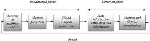
This section discusses the proposed ODMR-IoT and its modules in detail. The ODMR-IoT framework algorithm runs in "rounds" which represent pre-determined time intervals where each round consists of five phases these phases are: the neighbor discovery phase, the CHs (Cluster-Head) election phase, the cluster formation phase, the scheduling phase and the transmission phase (inter-cluster and intra-cluster).
For the neighbor discovery phase, each node at the end of this phase knows its neighbors. The clustering phase begins with the selection of cluster heads and the formation of clusters. During this phase, each node either elects itself a cluster-head or joins a cluster. Nodes with high value (Wch) can act as CH. The selection of CH is offered based on many factors. At the level of the ODMR-IoT, Figure 1.
The following factors are considered: the sum of the degrees of chauvochism with all these neighbors of a node, the residual energy, condition of distance from the fog, the weights of the factors such as the sum of the degrees of chauvochism, the residual energy, condition of distance from the forage determined in Eq. (2). To reduce collisions, each cluster-head generates a TDMA schedule. During the transmission phase, the data collected by the members of a cluster is sent to the neighbors to detect the context of outliers according to the TDMA schedule with multi-hop communication. The proposed mechanism is based on an initial set of data representing the first samples S to be detected by all the sensors (for example temperature or humidity).
A node's predecessor merges the data and sends it to using a multi-hop architecture as well. The proposed phases of ODMR-IoT are follow:
Figure 1. The proposed phases of ODMR-IoT
3.1.1 Discovery of neighbors phase
The neighbors discovery process is performed by a "Msg-Neighbors" message. The latter makes it possible to build neighbors tables thanks to a periodic exchange of messages necessarily containing the identifier of the sending node and its position. Any node j having received this message calculates the degree of chauvochism with this node based on the intersection between the two radiuses of the two sensors using the following formula Eq. (1).
lentille $=2 \mathrm{R}^{2} \operatorname{arrccos}\left(\frac{\mathrm{h}}{\mathrm{R}}\right)-2 * \mathrm{~h} \sqrt{\mathrm{R}^{2}-\mathrm{h}^{2}}$ (1)
where:
h is the distance between the two nodes divided by two.
R is the range of sensing of nodes.
If lentille is greater than zero, then node i is close to node j.so at the end each node saves the identifier and the coordinates of each of its neighbors and a lentille_sum which is the sum of the lentilles of all the Chauvochist neighbors with this node (Algorithm1).
|
Algorithm 1: Discovery of neighbor’s phase |
|
Input Msg-Neighbors; Output Degi, lentille_sum, Tneigh For i=1 to N do Broadcast of a message to nodes in its range; Decrease energy; For j=1 to N do If ( j receive the message ) then Decrease energy; Calculate lentille; If (lentille> 0 )then Calculate lentille; Add i to TNeigh; Lentille_sum←Lentille_sum+lentille; End End End End End |
3.1.2 Cluster-Head election phase
We have proposed the equation to choose the CH Eq. (2):
Wchi = α ∗Ei + β ∗(1/D) + δ ∗sum_lentille (2)
where, Ei is the residual energy, D is the distance to the fog node, sum_lentille: the sum of the degrees of chauvochism between the node and its neighbors and α, β, δ: are positive values.
To choose the CH each node i of the network uses Eq. (1) proposed to calculate the coefficient Wchi on which the election of the CH is based. A message is broadcast to these neighbors, this message includes its identifier and this coefficient. The receiving node compares its Wch value with all the neighboring nodes so it is self-elected as CH.
The election of the CH consists in each node i of the weight of each node. Then he broadcasts a message to these neighbors, this message includes its identifier and its Wch value. In this case each node can determine the node having the highest value of Wch. It compares its value of Wch with that of neighboring nodes. If node i has found its value from Ech greater than the value of all neighboring nodes, it is self-elected as a CH. Details are in Algorithm 2: CHs election.
The main objective of our protocol is to minimize the energy consumption, and to improve the detection accuracy for this reason our approach is based on the residual energy distance between the node and the fog for the selection of CHs. And to increase the efficiency of the detection, another parameter is considered: the degree of chauvochism of the node which represents the nodes which are in spatial correlation with this node can then generate values almost equal to that generated by this node. Below is the associated pseudo-algorithm algorithm 2:
|
Algorithm 2: CHs election |
|
Input Choice-CH, Ei, lentille_sum, Di,fog; Output Wi, Election of CH. Begin For i=1 to N do Caculate Wchi; Broadcast of a message to choice CH to each Neighbor; Decrease energy; If (Wchi>Wchj) then i←CH; Else j←CH; End If End For End |
3.1.3 Clusters formation phase
Each CH broadcasts a message with its non-CH neighbors containing its energy and its degree of chovochism. Each non-CH calculates a JC coefficient taking into consideration the energy of the CH and the sum of degree of shock "sum_lens" of CH, then it informs the CH of its decision. In the event of several membership proposals, this node must then determine which cluster it wants to belong to., it chooses the cluster-head with a maximum "JC" value.
JCch = Wch/Di,fog (3)
We have taken into consideration in this Eq. (3) the distance from the fog and the residual energy of this CH.
This equation allows the node to choose the CH which has a higher residual energy and which is the least distant from the fog.
|
Algorithm3: Clusters formation |
|
Input Ei lentille_sum, Di,fog, ; Output JChi, clusters formation. Begin For i=1 to N do If (i is a CH) then Broadcast of a message for cluster formation; Else i receive the message; add CH to the list of ch; calculate JC; sending Acceptation to CH having the maximal JC End If End For End |
3.1.4 Scheduling phase
(1) Intra-cluster scheduling
In this phase, each CH creates the TDMA table to allocate each member node a time slot for it to transmit its data. This schedule allows non-cluster leader nodes to go into sleep mode when they are not transmitting data to the cluster leader. Moreover, the use of TDMA approach in intra-cluster communications ensures that there are no data collisions in the cluster.
In our proposal we used a multi-hop routing between the CH and its members. Since the use of a single hop communication decreases the energy of the nodes. Where the nodes furthest from the CH die faster compared to the nodes closest. To improve and regulate the energy dissipation of distant nodes, it is proposed that the nodes communicate with their neighbors and not directly with the CH.
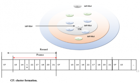
Before the creation of the TDMA table by the cluster-heads, each member node must determine its level in its cluster. Assigning a tier to each sensor node is done as follows: the CH has level 0 and the nodes having a collision with the CH are of level 1. Only the nodes which chauvinize with the CH can have this level. Then the nodes which have a clash with the level 1 nodes are level 2 nodes. The process continues for each cluster until the last level. If a node receives multiple messages it selects the message with the lowest level. At the end of this step each node can know its level and its predecessor and its successor Figure 2.
Figure 2. Intra-cluster scheduling
(2) Inter-cluster scheduling
To perform multi-hop routing between the CHs, it is necessary to ensure that each CH has their level relative to the other CHs. a message transmitted with a distance equal to 7m. the CH which has a distance less than 7m from the fog has level 1, After having determined the level 1 the neighboring CH (which have a distance < 7m), each CH determines its level which is level 2. The process is continuing until the last CH of the zone. For data transmission between the CHs, each CH chooses the nearest neighbor CH among its upper-level neighbor CHs.
3.1.5 Detection phase
The idea of outlier detection mechanisms proposed to analyze over time the detect data, for the detection of unexpected behaviors of a sensor node. The proposed mechanism is based on an initial set of data representing the first samples S to be detected by all the sensors (for example temperature or humidity) these data represent an initial situation without fault. The set of data is partitioned into two subsets, the first set D contains the data acquired by the sensors assuming that there is no fault situation and the second R stores the remaining samples. The first set S is used for the initial state estimation mechanism and the second set D is used for the detection phase. After the formation of the clusters, each member of the cluster self-estimates its status information in its slot. Status information is used for the detection of outliers
(1) State information estimation
Each sensor node self-estimates for a time slot duration ẟt its state (the min and max values) as indicated in the algorithm. If Xi represents a data vector detected by a sensor node i at time ẟt. The state information (min and max values) of i is calculated using the boxplot (the mustache method) method Eq. (4) and Eq. (5):
Min =Q1- 1.5*EIQ (4)
Max = Q3+ 1.5*EIQ (5)
where:
Q1: First quartile (Q1 or 25th percentile): also known as the lower quartile qn(0.25), is the median of the lower half of the Xi.
Q3: Third quartile (Q3 or 75th percentile): also known as the upper quartile qn(0.75), is the median of the upper half of the Xi.
EIQ: Interquartile range (IQR): is the distance between the upper and lower quartiles Eq. (6):
EIQ = Q3 - Q1 (6)
(2) Outliers detection and context identification
These states information is stored in current memory of the node (Min, Max). All times a new state information (NewMin, NewMax) of sensor node i is estimated and compared with the initial state information estimation (Min, Max), A n Alarm-Packet is sended to the predecessor node of sensornode i only if:
| Min − NewMin| >= threshod
or | Max − NewMax| >= threshod.
Each node i performs the sent of a message " Alarm-Packet (IDi, (NewMin, NewMax))" containing its identifier and the new state estimation. Any node j having received the message “Alarm-Packet”, calculates its new state estimation. If there is the same deviation in the state estimation it decides that the outlier is caused by a vent event else it decided that the sensed data is erroneous.
In the receiving of AlarmPacket: Algorithm 4
|
Algorithm 4: AlarmPacket reception |
|
Input AlarmPacket, sensed data, Min, Max, NewMin, NewMax; Output outlier a context identification. Begin Fori=1 to N do If (i receive AlarmPacket) then Eres (j) ←Eres(j) -ERx; If (|Min − NewMin| >= threshod or | Max − NewMax| >= threshod) then Sensed data is erroneous End End End For En |
To prove the performance of our proposed approach for IoT networks we went through a very important phase: the simulation phase. We present in this a simulation of an IoT network under NS3, to assess the performance of the ODMR-IoT protocol. This by comparing the results of our ODMR-IoT proposal with the two OPTICS protocols of [10, 25, 26], consists in transmitting all the detected data to the cluster leader for the identification of the aberrant context, and the UNICODE protocol of Bharti et al. [27] which consists in sharing the detected data between neighboring nodes for the identification of the aberrant context.
4.1 Evaluation metrics
The comparison of ODMR-IoT with UNICODE and OPTICS is made in terms of the following metrics:
4.1.1 Energy consumption
Calculate the energy consumed during the operation of the network to validate the adequacy of the ODMR-IoT. Energy consumption is calculated using the model proposed by Choi and Lee [28]. We have used the following equations to calculate the communication energy dissipations (Table 2):
Table 2. The model used to calculate the energy consumption
|
Communication |
Equation |
|
The energy consumed for the transmission of k-bits packets over the distance d |
ETx(K, d) = KEelc + KEampd (7) |
|
Energy expended to receive a packet of k-bits |
ERx(K) = KEelc (8) |
|
The residual energy of a node Ni, after transmission of a packet of k bits over distance d |
Eri= Einitial− (ETX(k, d) + ERX(K)) (9) |
|
The total initial energy of the network |
Etotal= NEinitial (10) |
|
The average energy of all live sensor nodes |
Eaverage = $\frac{\sum_{n=1}^{N} \text { Eresiduelle }(i)}{N}$ (11) |
4.1.2 Average latency
The average latency is defined as the number of slots, the latency includes the time between the transmission by the source and the last reception of the broadcast message. So the average latency is the average of the communication latencies of each node with its CH. If a packet sent from node i to its CH x via the following path:
i → n1 → n2 →... → nk → CHx
|
ODMR-IoT |
INCODE |
OPTICTS |
|
dti = slot (n1) + Tp |
dti = slot (nk) + Tp |
dti = slot (nk) + Tp |
Note that if a node i does not send data it has no latency therefore dti equal to 0 slots. Therefore the average communication latency in a cluster of size m is given as follows:
dt cluster $=\frac{\sum_{\mathrm{i} \in \text { cluster }} \quad \mathrm{dti}}{(\mathrm{m}-1)}$ (12)
Or:
i: represents the identifiers of the nodes.
m: represents the size of the cluster.
And the average latency per cluster in a hierarchical network is given in the formula:
$\mathrm{dt}=\frac{\sum_{\mathrm{i}=1}^{\mathrm{N}} \mathrm{dti}}{\mathrm{N}}$ (13)
i: represents the identifiers of the nodes.
N: represents the number of clusters in the network.
4.2 Network deployment
The simulation makes it possible to test, while minimizing the cost, the protocols proposed and to prevent the problems which could arise in the future to implement the technology that best meets the needs. to simulate our protocol we used the most widespread simulator in the field of networks which is NS3 (Network Simulator Version 3).
To test our protocol, we simulated a network of 53 nodes deployed in the Intel Bar kley laboratory. The sensor nodes are in a 2D space the coordinates (x, y) are given. It is assumed that our network topology will be divided into seven clusters (1 to 7) using algorithm1. After the execution of the cluster formation mechanism the resulting clusters are represented as follows (Table 3):
Table 3. Network deployment
|
cluster |
node |
Predecessor |
Level |
|
cluster3 |
15 |
16 |
3 |
|
14 |
18 |
2 |
|
|
16 |
17 |
2 |
|
|
22 |
21 |
2 |
|
|
17 |
19 |
1 |
|
|
18 |
19 |
1 |
|
|
20 |
19 |
1 |
|
|
21 |
19 |
1 |
|
|
19 |
0 |
0 |
|
|
cluster |
node |
Predecessor |
Level |
|
cluster4 |
24 |
25 |
4 |
|
23 |
27 |
4 |
|
|
25 |
26 |
3 |
|
|
26 |
28 |
2 |
|
|
27 |
28 |
2 |
|
|
28 |
31 |
1 |
|
|
29 |
31 |
1 |
|
|
30 |
31 |
1 |
|
|
32 |
31 |
1 |
|
|
31 |
0 |
0 |
|
|
cluster |
node |
Predecessor |
Level |
|
cluster5 |
1 |
5 |
2 |
|
33 |
4 |
1 |
|
|
34 |
4 |
1 |
|
|
35 |
4 |
1 |
|
|
36 |
4 |
1 |
|
|
39 |
0 |
0 |
|
|
37 |
11 |
2 |
|
|
cluster |
node |
Predecessor |
Level |
|
cluster6 |
42 |
39 |
2 |
|
39 |
40 |
1 |
|
|
41 |
40 |
1 |
|
|
43 |
40 |
1 |
|
|
40 |
0 |
0 |
|
|
cluster |
node |
Predecessor |
Level |
|
Cluster7 |
50 |
49 |
4 |
|
49 |
48 |
3 |
|
|
51 |
48 |
3 |
|
|
48 |
47 |
2 |
|
|
44 |
45 |
1 |
|
|
46 |
45 |
1 |
|
|
47 |
45 |
1 |
|
|
45 |
0 |
0 |
4.3 Dataset description and outlier(s) injection
An actual dataset from Intel [29] is used for our assessment. And to simplify, the experiments are based on temperature and leight values and we have not tested the other values. To model the scenario, the data set is modified by injecting outliers based on the scenario of Ref. [30].
4.4 Parameters set up
To evaluate the performance of our framework, we implemented the UNICODE framework and the OPTICS framework, under NS3. A comparison between the simulation results of the UNICODE, OPTICS and ODMR-IoT algorithms is performed. The UNICODE, OPTICS and ODMR-IoT algorithms is carried out. The simulation parameters are summarized in Table 4.
Table 4. Parameters set up
|
Fog emplacement |
(15,25) |
|
Number of nodes |
54 |
|
Network size |
40.5 X 40.5 |
|
Data packet size |
2000 Bytes |
|
Control packet size |
512 Bytes |
|
Initial energy |
4 Joules |
|
Ray of nodes |
3.5 mètres |
|
Threshold ℰ |
can be set as per the application requirement. |
|
ẟt |
13 minutes |
|
Simulation time |
500 Seconds |
4.4.1 The optimal values of α, β, δ
To choose optimal values of α, β, δ for the CH election we have run several experiments with different values of α, β, δ the election equation will become as follows (Table 5):
Table 5. The optimal values of α, β, δ
|
3 |
11,9105 |
3,97027 |
1,11803 |
0.3 |
0.2 |
0.5 |
7,32521708 |
|
4 |
15,7501 |
3,9539 |
5,59017 |
0.3 |
0.2 |
0.5 |
9,09699709 |
|
5 |
10,6758 |
3,97028 |
9,17878 |
0.3 |
0.2 |
0.5 |
6,55077339 |
|
6 |
13,9494 |
3,97028 |
8,01561 |
0.3 |
0.2 |
0.5 |
8,19073531 |
|
22 |
4,25078 |
3,96974 |
18,7417 |
0.3 |
0.2 |
0.5 |
3,32698339 |
|
2 |
4,85044 |
3,97027 |
4,5 |
0.3 |
0.2 |
0.5 |
3,66074544 |
4.5 Evaluation metrics
We used the quantitative F1 measurements to assess the detection accuracy of our protocol. The F1 score is given as follows:
$F 1=2 \times \frac{\text { recall } \times \text { precision }}{\text { precision }+\text { recall }}$ (14)
recall $=\frac{\mathrm{TP}}{\mathrm{TP}+\mathrm{FN}}$ precision $=\frac{\mathrm{TP}}{\mathrm{TP}+\mathrm{FP}}$ (15)
4.6 Accuracy evaluation
4.6.1 Event detection accuracy
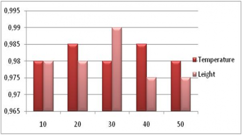
Figure 3 shows the event detection accuracy performance of the ODMR-IoT for various window sizes (tw). As the tw increases, the value of precision decreases because the large value of recall because the greater number of FPs and large tw size decreases the number of FNs.
Figure 3. Event detection accuracy
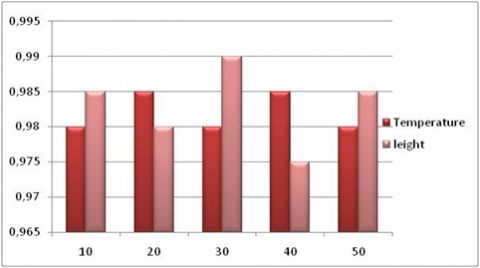
4.6.2 Erroneous data detection accuracy
Figure 4 shows the erroneous data detection accuracy. Similar to event detection accuracy, erroneous data detection accuracy also improves with the tw.
The OPTICS protocol the nodes shares the sensed data with these neighboring nodes, it shares each data point with the others, it requires the sharing of each detected data with the other nodes, the INCODE protocol the nodes shares the sensed data with these neighboring nodes, it does not share each data point with the others, it requires the sharing of each detected data with these neighboring nodes. However, ODMR-IoT les noueds does not share every sensed data with these neighbors, it shares except in case of outlier detection. We therefore take into account several metrics to evaluate the performance of our contribution [31].
Figure 4. Erroneous data detection accuracy
4.7 Effect on network parameters
4.7.1 Energy consumption
Figure 5. Energy consumption comparison
Considering the energy limitations of the sensors, it is essential to reduce the energy consumed at all levels in order to allow a longer lifetime of the network. It can be seen in the figures that the average residual energy of the three studied protocols decreases with the increase in the simulation time. This is due to the number of messages passing through the network. The simulations carried out show that the average residual energy at the level of the ODMR-IoT protocol is greater than the average residual energy at the level of INCODE and OPTIC. This is due in particular to the difference in the operating mode of the three protocols and the number of messages transmitted in the temp. This proves the contribution of the technique adopted for the formation of the clusters used. So the ODMR-IoT protocol balances the energy load thanks to the good distribution of the cluster-heads and the load balancing between the clusters, which ensures the improvement of the amount of the residual energy and consequently a longevity of the network. And the second cause, unlike INCODE and ODMR-IoT the nodes do not share every data point detected with neighboring nodes. However, ODMR-IoT does not require sharing the state estimate up to the cluster head, but it does require sharing it with its predecessor at the next level unlike INCODE where the nodes share the state estimate up to the cluster head. at the head of the cluster. (Figure 5).
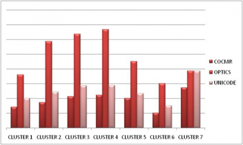
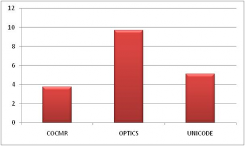
Average latency
Figure 6 illustrates the packet latency over the number of nodes. Latency is the time between sending by the source and the last reception of the broadcast message. The simulation results show that the ODMR-IoT protocol offers better results in terms of latency reduction unlike the INCODE and OPTICS protocol. Indeed, OPTICAL involves the transmission of detected data to the cluster head. In OPTICS each sensor node shares each sensed data with its neighboring nodes. Then the number of messages exchanged and the network traffic in the network increase that results packet collision, then end-to-end delay increased. (Figure 7).
Figure 6. Average latency by cluster
Figure 7. Average latency in the network
This article has discussed the outlier detection problem and its context for WSNs. We have proposed a new detection protocol based on the real-time analysis of the data collected by the sensor nodes. The model includes an algorithm for forming clusters and an algorithm for identifying outliers and the context of these outliers. In future work, we will improve our protocol to better address the problem of data privacy by using fog computing devices. Manage the mobility of the base station. Manage the mobility of nodes in the area. Consider the case of several base stations. Extending our protocol to a homogeneous environment. Using a combination of other metrics for CH election. Manage member node failure by introducing a mechanism allowing member failure detection by their cluster-head.
[1] Ayadi, A., Ghorbel, O., Obeid, A.M., Abid, M. (2017). Outlier detection approaches for wireless sensor networks: A survey. Computer Networks, 129: 319-333. https://doi.org/10.1016/j.comnet.2017.10.007
[2] D'Arienzo, M., Romano, S.P. (2019). A cost effective solution for the deployment of wireless sensor networks. International Journal of Mobile Network Design and Innovation, 9(2): 97-105. https://doi.org/10.1504/IJMNDI.2019.10027010
[3] Zhang, Y., Hamm, N.A., Meratnia, N., Stein, A., Van De Voort, M., Havinga, P.J. (2012). Statistics-based outlier detection for wireless sensor networks. International Journal of Geographical Information Science, 26(8): 1373-1392. https://doi.org/10.1080/13658816.2012.654493
[4] Gil, P., Santos, A., Cardoso, A. (2013). Dealing with outliers in wireless sensor networks: an oil refinery application. IEEE Transactions on Control Systems Technology, 22(4): 1589-1596. https://doi.org/10.1109/TCST.2013.2288519
[5] Hida, Y., Huang, P., Nishtala, R. (2004). Aggregation query under uncertainty in sensor networks. Department of Electrical Engineering and Computer Science. University of California, Berkeley.
[6] Bai, M., Wang, X., Xin, J., Wang, G. (2016). An efficient algorithm for distributed density-based outlier detection on big data. Neurocomputing, 181: 19-28. https://doi.org/10.1016/j.neucom.2015.05.135
[7] Lyu, L., Jin, J., Rajasegarar, S., He, X., Palaniswami, M. (2017). Fog-empowered anomaly detection in IoT using hyperellipsoidal clustering. IEEE Internet of Things Journal, 4(5): 1174-1184. https://doi.org/10.1109/JIOT.2017.2709942
[8] Gaura, E.I., Brusey, J., Allen, M., Wilkins, R., Goldsmith, D., Rednic, R. (2013). Edge mining the internet of things. IEEE Sensors Journal, 13(10): 3816-3825. https://doi.org/10.1109/JSEN.2013.2266895
[9] Xie, M., Hu, J., Guo, S., Zomaya, A.Y. (2016). Distributed segment-based anomaly detection with Kullback–Leibler divergence in wireless sensor networks. IEEE Transactions on Information Forensics and Security, 12(1): 101-110. https://doi.org/10.1109/TIFS.2016.2603961
[10] Abid, A., Masmoudi, A., Kachouri, A., Mahfoudhi, A. (2017). Outlier detection in wireless sensor networks based on optics method for events and errors identification. Wireless Personal Communications, 97(1): 1503-1515. https://doi.org/10.1007/s11277-017-4583-7
[11] Bharti, S., Pattanaik, K.K., Pandey, A. (2020). Contextual outlier detection for wireless sensor networks. Journal of Ambient Intelligence and Humanized Computing, 11(4): 1511-1530. https://doi.org/10.1007/s12652-019-01194-5
[12] Branch, J.W., Giannella, C., Szymanski, B., Wolff, R., Kargupta, H. (2013). In-network outlier detection in wireless sensor networks. Knowledge and Information Systems, 34(1): 23-54. https://doi.org/10.1109/ICDCS.2006.49
[13] Radivojac, P., Korad, U., Sivalingam, K.M., Obradovic, Z. (2003). Learning from class-imbalanced data in wireless sensor networks. In 2003 IEEE 58th Vehicular Technology Conference. VTC 2003-Fall (IEEE Cat. No. 03CH37484), 5: 3030-3034. https://doi.org/10.1109/VETECF.2003.1286180
[14] Rajasegarar, S., Leckie, C., Palaniswami, M., Bezdek, J. C. (2006). Distributed anomaly detection in wireless sensor networks. In 2006 10th IEEE Singapore international conference on communication systems, pp. 1-5. https://doi.org/10.1109/ICCS.2006.301508
[15] Giatrakos, N., Deligiannakis, A., Garofalakis, M., Kotidis, Y. (2020). Omnibus outlier detection in sensor networks using windowed locality sensitive hashing. Future Generation Computer Systems, 110: 587-609. https://doi.org/10.1016/j.future.2018.04.046
[16] Deligiannakis, A., Kotidis, Y., Vassalos, V., Stoumpos, V., Delis, A. (2009). Another outlier bites the dust: Computing meaningful aggregates in sensor networks. In 2009 IEEE 25th International Conference on Data Engineering, pp. 988-999. https://doi.org/10.1109/ICDE.2009.100
[17] Burdakis, S., Deligiannakis, A. (2012). Detecting outliers in sensor networks using the geometric approach. In 2012 IEEE 28th International Conference on Data Engineering, pp. 1108-1119. https://doi.org/10.1109/ICDE.2012.85
[18] Giatrakos, N., Deligiannakis, A., Garofalakis, M., Kotidis, Y. (2020). Omnibus outlier detection in sensor networks using windowed locality sensitive hashing. Future Generation Computer Systems, 110: 587-609. https://doi.org/10.1016/j.future.2018.04.046
[19] Gao, Q., Blow, K.J., Holding, D.J., Marshall, I.W., Peng, X.H. (2006). Radio range adjustment for energy efficient wireless sensor networks. Ad Hoc Networks, 4(1): 75-82. https://doi.org/10.1016/j.adhoc.2004.04.007
[20] Bosman, H.H., Iacca, G., Tejada, A., Wörtche, H.J., Liotta, A. (2017). Spatial anomaly detection in sensor networks using neighborhood information. Information Fusion, 33: 41-56. https://doi.org/10.1016/j.inffus.2016.04.007
[21] Deng, X., Jiang, P., Peng, X., Mi, C. (2018). An intelligent outlier detection method with one class support tucker machine and genetic algorithm toward big sensor data in internet of things. IEEE Transactions on Industrial Electronics, 66(6): 4672-4683. https://doi.org/10.1109/TIE.2018.2860568
[22] Titouna, C., Naït-Abdesselam, F., Khokhar, A. (2019). DODS: A distributed outlier detection scheme for wireless sensor networks. Computer Networks, 161: 93- https://doi.org/101.0.1016/j.comnet.2019.06.014
[23] Dau, H.A., Ciesielski, V., Song, A. (2014). Anomaly detection using replicator neural networks trained on examples of one class. In Asia-Pacific Conference on Simulated Evolution and Learning, pp. 311-322. https://doi.org/10.1007/978-3-319-13563-2_27
[24] Sheng, B., Li, Q., Mao, W., Jin, W. (2007). Outlier detection in sensor networks. In Proceedings of the 8th ACM International Symposium on Mobile Ad Hoc Networking and Computing, pp. 219-228. https://doi.org/10.1145/1288107.1288137
[25] Lyu, L., Jin, J., Rajasegarar, S., He, X., Palaniswami, M. (2017). Fog-empowered anomaly detection in IoT using hyperellipsoidal clustering. IEEE Internet of Things Journal, 4(5): 1174-1184. https://doi.org/10.1109/JIOT.2017.2709942
[26] Shahid, N., Naqvi, I.H., Qaisar, S.B. (2012). Real time energy efficient approach to outlier & event detection in wireless sensor networks. In 2012 IEEE International Conference on Communication Systems (ICCS), pp. 162-166. https://doi.org/10.1109/ICCS.2012.6406130
[27] Bharti, S., Pattanaik, K.K., Pandey, A. (2020). Contextual outlier detection for wireless sensor networks. Journal of Ambient Intelligence and Humanized Computing, 11(4): 1511-1530. https://doi.org/10.1007/s12652-019-01194-5
[28] Choi, S.H., Lee, K.O. (2011). A cluster based energy efficient location routing protocol in wireless sensor networks. Institutional Repository UIN Syarif Hidayatullah Jakarta. http://repository.uinjkt.ac.id/dspace/handle/123456789/28252.
[29] Intel Lab Data (2014). http://db.csail.mit.edu/labdata/data.txt.gz, accessed on 14 November 2014.
[30] Nesa, N., Ghosh, T., Banerjee, I. (2018). Non-parametric sequence-based learning approach for outlier detection in IoT. Future Generation Computer Systems, 82: 412-421. https://doi.org/10.1016/j.future.2017.11.021
[31] Deepika, N., Nirupamabhat, M. (2020). An optimized machine learning model for stock trend anticipation. Ingénierie des Systèmes d’Information, 25(6): 783-792. https://doi.org/10.18280/isi.250608