Shiva Prasad Satla* | Manchala Sadanandam | Buradagunta Suvarna
© 2020 IIETA. This article is published by IIETA and is licensed under the CC BY 4.0 license (http://creativecommons.org/licenses/by/4.0/).
OPEN ACCESS
Many vulnerable, heinous acts that are coming about in the society especially at Roads, most specifically affecting women in the society, are more in recent days. Though new technologies are developing day by day, the fatality rate is not in control to date. Without proper guidance to the people about the particular place where there is a big scope of occurrence of a greater number of accidents, this menace cannot be regulated. It is required to highlight the District-wise data and Roads where the accidents and fatalities are more. The data would help the policymakers to put in place Focused Initiatives regarding those top dangerous roads to address the menace of rising road accidents and resultant fatalities. In this, we created a dataset in Andhra Pradesh where we include those attributes that are helpful for our analysis to predict which road is the most dangerous one. We applied various Machine Learning models such as Logistic regression, Random forest classifier, Gradient Boosting Classifier, Gaussian Naive Bayes, Decision Tree Classifier, K- Nearest Neighbour Classifier and SVM to predict the dangerous roads. It is observed that Logistic Regression provides good accuracy with 87.14.
dangerous roads, support vector machine, accidents, fatalities, logistic regression, decision tree, random forest, gaussian naive bayes, K- nearest neighbor
Our country, India, unfortunately, ranks at the top with the highest number of fatalities with about 11% share in the world, in which Andhra Pradesh continues its rank with 7th position in India since 2015. Thus, this issue must be most important to the government to find the root cause of the accidents mainly on roads. For the very safety of citizens, governments of various states and local bodies of a number of districts can make use of this system to generate reports and find solutions for their citizens.
If the Government make the best use of this system and let its citizens, the Dangerous Roads, across the state, then while travelling, everyone prefer to take more no of precautions like maintaining the speed limit, avoiding night travels, etc. at maximum, rather they avoid that route and find an alternative road. This data also helps strangers, migrants, etc. to know the best paths to travel in the state, without any fear of threatening the journey. Above all, if one does not beware of the situations taking place daily in the society, and act blindly without any preventive measures, no government and not technology save him/her.
Accidents re happened due to various reasons in the world. In this alcohol consumptions, Curves in roads, Weather conditions, Traffic problems, Over speed like. In this, we considered one of the major reasons to get accidents is roads position and number of lanes. IN this we re-identified the some of the roads in A.P are dangerous where a greater number of accidents are taken place. We are collected different roads where the numbers of accidents are high. If the number of accidents is crossed more than 3K we can call as dangerous roads. Otherwise, it is a non dangerous road. When the people are moving in the rod they may be followed little care while driving. This Dataset is used for the people to give guidance that how they will drive along with the road. There are lot of roads are categorized as dangerous day by day that illustrated in Figure 1.
Figure 1. Illustration of dangerous roads
Accident prediction has been widely concentrated in the last 10 years. Generally, binomial regression was utilized to anticipate the number of accidents that happened on a road [1]. From the last 10 years, there are a lot of machine learning models that have evolved to predict accidents [2-4]. To predict they used features like temperature, weather, traffic, etc.
Najjar et al. [2] used BR and ANN to predict the accidents in Taiwan. They consider long one-year data on-road segments. The dataset they considered from 1997-98 which brought about 1,338 accidents. They observed ANN furnishes better outcomes with precision of 61.4% than BR. By utilizing the same dataset, Chang et al. [3] applied choice trees for the forecast of an accident. They utilized normal day by day traffic and the number of days with precipitation are the highlights. It delivers an exactness of 52.6%.
Lin et al. [4] utilized Frequent Pattern trees and Random Forest for the expectation of accidents. They utilized the KNN and Bayesian system for constant accidents expectation on a fragment of a highway. Using the mean and at times the standard deviation of the climate condition, the detectable quality, the traffic volume, the traffic speed, and the inhabitants evaluated during the last very few minutes their models predict the event of an accident. They procured the best results using the Frequent Pattern trees to incorporate decisions and achieved a precision of 61.7%. It should be seen that they used only a little case of the possible negative models, to oversee data unevenness.
Chang [5] applied different methods that are used to find the frequency of accidents happened in that road by using binominal and ANN methods. Yuan et al. [6] used to predict accidents are neural networks, decision trees, and a hybrid model using a neural network and decision tree. They acquired the best exhibitions with the hybrid model that produced the 90% accuracy for the expectation of lethal wounds. They distinguished the safety belt use, liquor combination, and light conditions of the driver considered as highlights. Frequent patterns tree method was applied by Wilson [7] who find the most frequent patterns caused for accidents. Theofilatos [8] likewise utilized ongoing information on 2 urban arterials of Athens city to examine street accident probability and seriousness. They used logistic regression and Random Forest for accident prediction. The most significant highlights distinguished were the coefficients of variation of the flow per lane, the speed, and the inhabitants. Moreover, numerous examinations target foreseeing the seriousness of an accident utilizing different data from the mishap all together to comprehend what makes an accident be lethal.
Chen et al. [1] likewise considered car crash seriousness by taking a gander at the choice principles of a decision tree utilizing a database of 1,801 expressway accidents. They identified that reason for the accident, the light poison, the gender of the driver, the climate were the most significant highlights. These investigations utilize generally little datasets utilizing information from just a couple of years or just a couple of streets. In reality, it can be difficult to gather all the fundamental data to perform street mishap expectations for a bigger scope, and managing huge datasets is progressively troublesome and geospatial analysis for accidents also explained by Gorelick et al. [9]. Be that as it may, later examinations [10-12] performed a mishap forecast at a lot bigger scope, typically utilizing profound learning models. Profound learning models can be prepared on the web with the goal that the entire dataset doesn't have to remain in memory. This makes it simpler to manage enormous datasets.
Chen et al. [10] utilized human versatility data collected from cell phone GPS information and chronicled accident records to assemble a model for the ongoing expectation of auto collision hazard in zones of 500 by 500 meters. The hazard level of a territory is characterized as the aggregate of the seriousness of mishaps that happened in the territory during the hour. Their model accomplishes a Root Mean-Square Error (RMSE) of 1.0 mishap seriousness. They thought about the exhibition of their profound learning model with the exhibitions of a couple of old-style AI calculations: Decision Tree, LR, and SVM, which all deteriorated RMSE values of individually 1.41, 1.41, and 1.73. they have not used the Random Forest calculation while it typically has great expectation exhibitions.
Abdullah and Emam [13] are applied the big data methodology to analyze the traffic accidents by applying the map reduced procedure and Augmented reality technology is applied by Calvi et al. [14]. In this authors are applied the augmented reality technique at zebra crossing where the peoples need to cross the roads. This techniques provides the basic information at the zebra crossing to the drivers to take necessary precautions to reduce the accidents. To reduce the accidents and severity of accidents Gaylor et al. [15] analyzed the airbags and its working in their work. Experience will also used to reduced the accidents along the roads. Miyaji et al. [16] are prepared the questionnaires to the drivers to know the situations and different conditions when there are more accidents will be happened.
In this we have taken, the social issue of deaths in the society, due to dangerous roads especially, with lack of necessary precautions entitled on the boards, so that we suggest government bodies to take absolute preventive measures in order to reduce the accidents at the respective dangerous Roads and to make this process computerized by implementing principles of data mining and analytics. The government is collecting data only in its raw format that the number of deaths that are happening across the country due to various reasons among which we are using the accidents that are correlated to roads in Andhra Pradesh. We collected this data from different roads in A.P. It may help to Government bodies and people to know the accident-prone areas and we apply different machine learning models. Predicting a dangerous Road involves, considering more no of factors, where we confine our dataset with few elements that are known to everyone.
Table 1. Different roads and sample database values
|
Name of the road |
District |
road accedients |
girls harazments |
Theft |
Total |
status |
|
National highway 360a |
Srikakulam |
5014 |
111 |
469 |
5594 |
1 |
|
Ichchapuram - Sompeta road |
Srikakulam |
3014 |
157 |
914 |
4085 |
1 |
|
Kotturu - Palakonda road |
Srikakulam |
7801 |
99 |
140 |
8040 |
1 |
|
Nandhigam – Narasannapeta (NH_5) |
Srikakulam |
6152 |
177 |
119 |
6448 |
1 |
|
Ponduru - Ko0haram road |
Srikakulam |
1564 |
32 |
147 |
1743 |
0 |
|
Hiramandalam - Patapatnam junction |
Srikakulam |
2014 |
209 |
149 |
2372 |
0 |
|
Tenali - guntur (via Narakoduru road) |
Guntur |
1596 |
118 |
301 |
2015 |
0 |
|
Narasaraopeta - Sathenapalli road |
Guntur |
4217 |
369 |
412 |
4998 |
1 |
|
Guntur - Mangalagiri (NH-5) |
Guntur |
2590 |
471 |
601 |
3662 |
1 |
|
Vijayawada - Amaravathi Road |
Guntur |
2659 |
259 |
301 |
3219 |
1 |
|
Bapatla - Repalle (NH-214A) |
Guntur |
1470 |
214 |
214 |
2154 |
0 |
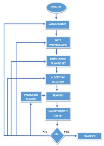
The system will analyze data in two phases, using a classifier for each phase. Data will be used for both training and testing purposes. The extracted data includes records for accidents due to vehicles, theft cases, girl harassment cases that happened at various Roads in all districts of Andhra Pradesh. 70 percent of the data will be used for training the system, and the remaining 30 percent of the data will be used for testing the accuracy of the system. Working procedure followed in this as shown in Figure 2 and Table 1 provides the sample data that are collected from different regions in Andhra Pradesh.
Figure 2. Methodology followed in identifying dangerous prediction in roads
3.1 Database creation
Data can originate from different sources and needs to be checked before it can be put to use. This can be done by directly importing files that may already be available in .csv or .xlsx formats. The attributes we used in the dataset are Name of the Road, Name of the District, no of theft cases registered, No of Girls Harassment cases registered, No of Vehicle accidents registered, Total No of Accidents Registered at that particular Road, Status of the Road whether it is Dangerous or not. Further, under these attributes, we include 113 roads in Andhra Pradesh. Figure 3 shows the description of data types of attributes and the sample database collected for prediction.
Figure 3. Number of attributes used in the creation of a database
The database contains two classes DANGEROUS which is indicated by “1” and NON-DANGEROUS indicated by “0”. We took 3000 (accidents) as a cut-off limit to segregate the dangerous and non dangerous roads list. That means, the roads where the total number of accidents are greater than 3000, then they will be categorized as Dangerous and the rest as non- Dangerous.
3.2 Data pre-processing
Datasets in any data mining application can have missing data values. These missing values can get propagated due to a lack of communication among the parameters in a data collection system. These missing values can affect the performance of a data mining system, and it should be noticed. In this we have to deal with imbalanced data contained dangerous and non dangerous roads. The mining model clearly differentiate this data and identify the dangerous roads. If number of accidents more than 3k we are making that road as dangerous road otherwise it is not a dangerous road.
Figure 4 provides the procedure applied in data preprocessing. In database we are concentrate on three aspects theft, road accidents and girls harassment. Girls harassments are considered new in this work because it is very essential today's situation at outside because DISHA case is a real example for this. If we provide enough information to police or public then people will more care in that particular roads. More strict rules will be imposed on the way, for that we are consider the girls harassment and also theft is also important to predict how the road is and is there any chance to happened to unknown things on the roads. This is my research sample we are considered to predict the dangerous road.
Figure 4. Data pre-processing
Classification algorithms seem the most appropriate type of algorithms to implement our proposed solution. Classification refers to the task of giving a machine learning algorithm features and having the algorithm put the instances/data points into one of many discrete classes. Classes are categorical in nature; it isn't possible for an instance to be classified as partially one class and partially another.
There are two phases in the prediction of dangerous roads i.e.
Phase I
In the first phase of the system, it comprises of extraction of data related to parameters required for Roads classification, which are Theft cases, Girls Harassment cases, and accidents. This data will then be standardized to have a consistent format and loaded into the database.
The analysis of this data will produce results with other parameters, which can be used to calculate the probability of a road to become a dangerous road and classifying it as various levels of danger.
Steps followed in Phase I
1. Extract the data from available places.
2. Transform the data into a standard format and then load it into the database.
2.1 Analysing the theft data
2.2 Analysing the accidents data
2.3 Analysing the girl harassment data
2.4 Analysing the total no of accidents at the particular road
3. Correlation analysis for dangerous road prediction.
4. End Phase I.
Phase II
The phase two of the system will obtain the result and attributes from phase one and feed it into the next classifier.
Steps followed in Phase II
1. Start the phase II.
2. Obtain the dangerous road prediction from phase1.
3. Generate reports for users.
4. End of phase II.
The algorithms that we will be making use are as follows:
4.1 Logistic regression
It is very powerful method for binary classification. It is a straightforward calculation that performs very well on a wide scope of issues. The name of this calculation is strategic relapse as a result of the strategic capacity that we use in this calculation. This strategic capacity is characterized as:
predicted=1/(1+e-x)
The calculated relapse model takes genuine esteemed information sources and makes a forecast with respect to the probability of the information having a place with the default (class 0). In the event that the probability is > 0.5 we can accept the yield as an expectation for the default (class 0), in any case, the forecast is for the different (class 1) as shown in Figure 5.
Figure 5. Strategic capacity
Logistic regression in our work produced 87.8% because it is perfectly working for the binary classification models. In our problem also we consider the problem like dangerous and non dangerous roads consider class 0 and class 1. The advantage of LR models easy to implement and not required much mathematical computations. It is not needed or setting parameters, if we change any variable which is not related to the output variable also it will work well but it is not applicable to the non liner problems.
4.2 Random forest
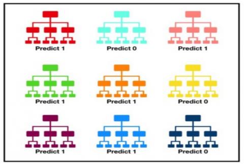
Random forest, similar to its name recommends, involves progressively singular decision trees that works as a group. Each individual tree in the random forest lets out a class estimate and the class with the most votes transforms into our model's desire. The essential thought driving arbitrary backwoods is a fundamental anyway stunning one the adroitness of gatherings. In data science talk, the clarification that the self-assertive forest area model works so well is innumerable modestly uncorrelated models (trees) functioning as a leading group of trustees will beat any of the individual constituent models. The reason behind this eminent effect is that the trees shield each other from their individual errors. The advantage of this model is easily identify the test error if any is there in the model without considerer the cost of training model with repletion. Different types of RF as shown in Figure 6. The drawback this model is it reduces the performance when the problem is complex. If the data size is more it will give less performance.
Figure 6. Different types of random forests
4.3 Gradient boosting classifiers
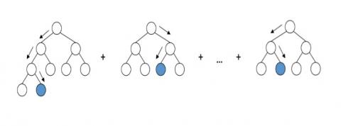
Gradient boosting classifiers are a gathering of machine learning calculations that join numerous feeble learning models together to make a solid prescient model. Choice trees are normally utilized while doing gradient boosting. Gradient boosting models are turning out to be well known on account of their viability at characterizing complex datasets. The working of the GBC method as shown in Figure 7.
In this Gradient boosting, you look a gander at all the perceptions that the machine learning calculation is prepared on, and you leave just the perceptions that the machine learning technique effectively grouped behind, stripping out different perceptions. Another powerless student is made and tried on the arrangement of information that was ineffectively grouped, and afterward simply the models that were effectively characterized are kept. The advantage of this model is very flexible model means it will not require the preprocessing also. It will work for all the databases. The drawback of this method is takes longer time to construct tress with complex data.
Figure 7. Basic working of gradient boosting
4.4 Gaussian Naive Bayes algorithm
A Gaussian Naive Bayes algorithm is a unique type of NB calculation. Bayes' theorem is dependent on restrictive likelihood. The contingent probability helps us computing the likelihood that something will occur, given that something different has just occurred. Depending upon the likelihood score they divide the roads as shown in Figure 8.
Gaussian Naive Bayes calculation is explicitly utilized when the highlights have consistent qualities. It's likewise expected that all the highlights are following a Gaussian dissemination i.e. normal distribution. The drawback this algorithm is zero probability problem. The occurrence probability of any attribute is zero then it reduces the prediction capacity. This model is it assume that all the attributes are independent but it is not happened most of the case even in this work also we are considered accidents and harassments are collectively identify the dangerous roads.
Figure 8. Division of class labels
4.5 Decision trees
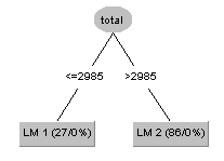
Decision trees a kind of Supervised Machine Learning where the information is ceaselessly part as indicated by a specific parameter. In choice investigation, a choice tree can be utilized to outwardly and unequivocally speak to choices and dynamic. The tree can be clarified by two elements, specifically choice hubs and leaves. The leaves are the choices or the ultimate results as shown in Figure 9. Also, the choice hubs are the place the information is part.
Decision trees gain from information to surmised a sine bend with a lot of on the off chance that else choice principles. The more profound the tree, the more perplexing the choice guidelines and fitter the model. The drawback of Decision tree is if data contains the noise or missing data then it can be easily over fitted. If we change single parameter then entire structure automatically changed. It will be produced bad results when it is over fitted even it produced good results in training.
Figure 9. Decision tree for two class labels
4.6 K-nearest neighbor (KNN) classification
It is a non-parametric and lethargic learning calculation. Non-parametric methods the model structure decided from the dataset. Lethargic calculation implies it needn't bother with any preparation information focuses for model age. All preparation information utilized in the testing stage. This makes preparing quicker and testing stage increasingly slow. Exorbitant testing stage implies time and memory. In the most pessimistic scenario, KNN needs more opportunity to check all information focuses and filtering all information focuses will require more memory for putting away preparing information.
K is the quantity of closest neighbors. The quantity of neighbors is the center central factor. K is commonly an odd number if the quantity of classes is 2. When K=1, at that point the calculation is known as the closest neighbor calculation shown in Figure 10. The drawback of KNN is it is sensitive to the Noise. If there is any noisy data is present then the performance is decreased.
Figure 10. Basic working KNN model
4.7 Support vector machine
Support Vector Machine is a supervised Machine Learning Algorithm which can be utilized for both arrangement and relapse difficulties. Be that as it may, it is for the most part utilized in characterization issues. In the SVM calculation, we plot every datum thing as a point in n-dimensional space (where n is number of highlights you have) with the estimation of each component being the estimation of specific arrange. At that point, we perform arrangement by finding the contrast between two classes quite well shown in Figure 11. This algorithm works for all kinds of data but drawback of SVM is it will reduce the performance when the data non-linear separable in input space. Above all methods are implemented in python jupyter notebook technology. Here we are showing the preprocessing steps done in python that used for all the models. The main research sample consider in this work is Girls harassment, Theft and road accident in that particular road. We collected 5,899 data samples from different sources to carried out research work.
Figure 11. Linear separation of class label
Identifying no of Districts in our database given in Figure 12 and assign the unique numbers for each road is depicted in Figure 13.
Figure 12. Identifying no of districts
Figure 13. District mappings
The data base that we are collected given to the model and the number of roads is shown in Figure 14 and status of roads either danger or not shown in Figure 15. The pictorial representation of dangerous and non-dangerous roads is plotted in Figure 16.
Figure 14. Identifying no of roads
Figure 15. Identifying no of dangerous and non-dangerous roads
Figure 16. Classifying dangerous & non-dangerous roads by plotting them in a graph
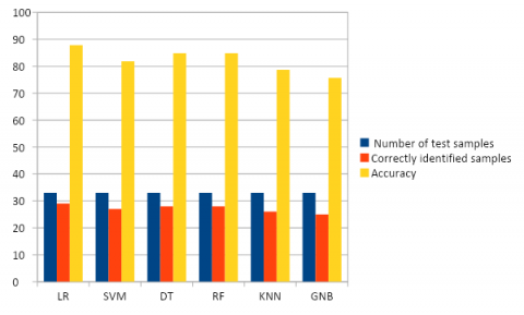
From Table 2, it is observed that logistic regression provides the good results. To find out the accuracy of a model we are applied 70% training and 30% for testing purpose. Accuracy of a model can be calculated as like code we are used is preprocessing of database what we created. In this first we assigning the unique numbers to unique roads in Andharapradesjh what we are collected in database. We are converting the nominal data to numeric to work out all the models. We are considered the number of accidents greater than 3000 it is dangers roads for this we collected information about 113 roads in A.P.
Accuracy = n/N where N is the number of testing samples and n is the correctly classified samples by model. In the above table we are given as number of accidents, weather conditions, ages of driver, girls harassment and theft happened in that road as input as input then model by using their classification rules it identified road is danger or not. The following Figure 17 shows the correctly identified samples.
Table 2. Description of the accuracy of various model
|
Classification model |
Number of test samples |
Correctly identified samples |
Accuracy |
|
Logistic Regression |
33 |
29 |
87.8 |
|
Support Vector machine |
33 |
27 |
81.8 |
|
Decision tree |
33 |
28 |
84.8 |
|
Random Forest |
33 |
28 |
84.8 |
|
KNN |
33 |
26 |
78.7 |
|
Gaussian Naive Bayes |
33 |
25 |
75.7 |
Figure 17. Visualizing the accuracy of various classifiers through classifier algorithm
Where we can observe here, that all classifiers predict the road registered with 1614 cases, as non-dangerous road & the road registered with 4285 cases as Dangerous road respectively.
In this paper, we predict the Dangerous Roads. In this, we have two classes as Dangerous and non-Dangerous and it is identified by using the data of the previous decade. So that, when the data reached the Government, it can take all those Road safety measures at the respective Dangerous roads. Actions are used to reduce the probability of accidents that took place at those Dangerous Roads. We applied different machine learning models to predict and Logistic regression is provided good accuracy with 87.8 compared to all other models. We wish to add more attributes to it and to have more accurate results. Hence, after testing on a set of attributes, we hope to extend the scope of the project by joining the attributes like the state of the country, no of curves/ U-turns, wild animal attacks at those particular roads across the country. These parameters may improve the accuracy. Unsupervised clustering to label data for classifiers will also improve accuracy, instead of using fixed intervals for the same.
[1] Chen, Q., Song, X., Yamada, H., Shibasaki, R. (2016). Learning deep representation from big and heterogeneous data for traffic accident inference. In Proceedings of the Thirtieth AAAI Conference on Artificial Intelligence (AAAI), pp. 338-344.
[2] Najjar, A., Kaneko, S., Miyanaga, Y. (2017). Combining satellite imagery and open data to map road safety. Proceedings of the Thirty-First AAAI Conference on Artificial Intelligence (AAAI), pp. 4524-4530.
[3] Chang, L.Y. (2005). Analysis of freeway accident frequencies: Negative binomial regression versus artificial neural network. Safety Science, 43(8): 541-557. https://doi.org/10.1016/j.ssci.2005.04.004
[4] Lin, L., Wang, Q., Sadek, A.W. (2015). A novel variable selection method based on frequent pattern tree for real-time traffic accident risk prediction. Transportation Research Part C: Emerging Technologies, 55: 444-459. https://doi.org/10.1016/j.trc.2015.03.015
[5] Chang, L.Y., Chen, W.C. (2005). Data mining of tree-based models to analyze freeway accident frequency. Journal of Safety Research, 36(4): 365-375. https://doi.org/10.1016/j.jsr.2005.06.013
[6] Yuan, Z., Zhou, X., Yang, T. (2018). Hetero-convLSTM: A deep learning approach to traffic accident prediction on heterogeneous spatio-temporal data. In Proceedings of the 24th ACM SIGKDD International Conference on Knowledge Discovery & Data Mining (SIGKDD), New York, USA, pp. 984-992. http://doi.acm.org/10.1145/3219819.3219922
[7] Wilson, D. (2018). Using machine learning to predict car accident risk. https://medium.com/geoai/using-machine-learning-to-predict-car-accident-risk-4d92c91a7d57, accessed on Apr. 16, 2020.
[8] Theofilatos, A. (2017). Incorporating real-time traffic and weather data to explore road accident likelihood and severity in urban arterials. Journal of Safety Research, 61: 9-21. https://doi.org/10.1016/j.jsr.2017.02.003
[9] Gorelick, N., Hancher, M., Dixon, M., Ilyushchenko, S., Thau, D., Moore, R. (2017). Google earth engine: Planetary-scale geospatial analysis for everyone. Remote Sensing of Environment, 202: 18-27. https://doi.org/10.1016/j.rse.2017.06.031
[10] Chen, C., Breiman, L. (2004). Using random forest to learn imbalanced data. University of California, Berkeley.
[11] Jia, Y., Shelhamer, E., Donahue, J., Karayev, S., Long, J., Girshick, R., Guadarrama, S., Darrell, T. (2014). Caffe: Convolutional architecture for fast feature embedding. In Proceedings of the 22nd ACM International Conference on Multimedia, 675-678. ACM. https://doi.org/10.1145/2647868.2654889
[12] Qin, W.Y., Liu, X., Kong, Z.B. (2018). analysis of characteristics of road traffic accident casualties in guilin. Open Journal of Social Sciences, 6(6): 90-96. https://doi.org/10.4236/jss.2018.66009
[13] Abdullah, E., Emam, A. (2015). Traffic accidents analyzer using big data. 2015 International Conference on Computational Science and Computational Intelligence (CSCI), Las Vegas, NV, USA, pp. 392-397 https://doi.org/10.1109/CSCI.2015.187
[14] Calvi, A., D’Amico, F., Ferrante, C., Ciampoli, L.B. (2020). Effectiveness of augmented reality warnings on driving behaviour whilst approaching pedestrian crossings: A driving simulator study. Accident Analysis and Prevention, 147: 105760. https://doi.org/10.1016/j.aap.2020.105760
[15] Gaylor, L., Junge, M., Abanteriba, S. (2019). Effectiveness of vehicle passive safety systems in lateral fixed-object collisions. International Journal of Vehicle Safety, 10(3-4). https://doi.org/10.1504/IJVS.2018.097705
[16] Miyaji, M., Danno, M., Oguri, K. (2008). Analysis of driver behavior based on experiences of road traffic incidents investigated by means of questionnaires for the reduction of road traffic accidents. International Journal of ITS Research, 6(1): 47-56.