Lingyan Ou* | Ling Chen
© 2020 IIETA. This article is published by IIETA and is licensed under the CC BY 4.0 license (http://creativecommons.org/licenses/by/4.0/).
OPEN ACCESS
With the rapid advances of Internet technology, some listed companies choose to disclose their financial information in the form of corporate internet reporting (CIR). However, there is little report on the risk factors and formation mechanism of CIR risks. To better prewarn, prevent and regulate CIR risks, this paper designs an CIR risk propagation model based on fuzzy neural network (FNN). Firstly, an evaluation index system (EIS) was established for CIR safety, and subject to fuzzy comprehensive evaluation (FCE), after reliability analysis and weighting of the indices. Based on the evaluation results, the hypotheses and risk propagation mode were summarized, and used to set up a risk propagation model. Finally, a neural network (NN) algorithm was created to predict the CIR risk propagation path. The proposed model and algorithm were proved effective through experiments. The research findings provide a novel tool to dig deep into the propagation mechanism of CIR risks.
corporate internet reporting (CIR), risk propagation, fuzzy neural network (FNN), evaluation index system (EIS)
The rapid advances of Internet technology have greatly changed the financial information disclosure. Some listed companies choose to disclose their financial information in the form of corporate internet reporting (CIR) on various online platforms [1-4]. Compared with traditional paper report, the CIR is open, transparent, and standardized, providing a wide audience with sufficient information in time. Like other online information, the CIR also faces various risks, which are amplified by people’s behaviors, values, interpretation, and association [5-9].
There are at least two kinds of CIR risks: the objective loss of participants on the information transmission chain, and the negative impacts of cultural and social factors involved in the disclosure [10-14]. Chen [15] constructed an evaluation index system (EIS) for CIR quality, evaluated the CIR quality of a listed company in northeastern China’s Liaoning Province, and put forward some improvement measures, highlighting the ability of extensible Business Reporting Language (XBRL) to automatically exchange and extract financial information in any software and information system, and make financial information more reliable and accurate. Tsantekidis et al. [16] studied the propagation mechanism of systemic financial risks, sorted out the influencing factors of systemic risks, and gave corresponding prevention suggestions.
The CIR in XBRL enables convenient and quick search, extraction, analysis, sharing, and mining of high-quality financial information. However, the ability to prevent and control CIR risks needs to be further enhanced in actual application [17-23]. Cakra and Trisedya [24] compared XBRL with Electronic Data Interchange (EDI) in operation mechanism and technical features, and summarized the positive effects of Internet security techniques, e.g. Internet protocol, encryption technology, digital signature, and virtual private network (VPN), on the implementation of XBRL. Shan [25] identified and classified the risk factors of XBRL CIR of wind power companies, constructed a Net draw-based network model of the risk propagation path, and controlled the CIR risks in the disclosure phase and the decision-making phase.
The existing studies on risk propagation path mainly tackle the maintenance of systematic financial security, and the financial security of largescale engineering projects. Only a few scholars have explored the influencing factors and formation mechanism of CIR risks. Moreover, there is little report that evaluates CIR risks, in virtue of the strengths of neural networks (NNs) in adaptation and self-learning. To improve the effectiveness and accuracy of risk warning, crisis prevention and financial supervision of the CIR, this paper presents a risk propagation model of the CIR based on fuzzy neural network (FNN).
The remainder of this paper is organized as follows: Section 2 constructs an EIS for CIR safety, performs reliability analysis and weighting of the indices, and makes a fuzzy comprehensive evaluation (FCE) of the EIS; Section 3 summarizes the hypotheses and risk propagation mode based on the evaluation results, and derives the risk propagation model in a systematic manner; Section 4 builds up a backpropagation NN (BPNN) algorithm capable of predicting the risk propagation path of the model, and specifies the training process of the network; Section 5 verifies the effectiveness of the proposed model and algorithm; Section 6 puts forward the conclusions of this research.
2.1 EIS construction
The EIS of CIR safety is the prerequisite for exploring the propagation mechanism of CIR risks. Considering the various objectives of CIR safety evaluation, some CIR safety indices were synthetized as per the design principle of CIR system, and in accordance with the requirements of documents like Electronic Information Disclosure Specification for Listed Companies and Classification of Information Disclosure for Listed Companies. In this way, a four-layer EIS was established for CIR safety, including three primary indices: CIR information security, CIR tool security, and CIR security system. Each primary index has several secondary and tertiary indices. The hierarchical EIS is detailed as follows:
The first layer (goal):
A={CIR safety}.
The second layer (primary indices):
A={A1, A2, A3}={CIR information security, CIR tool security, CIR security system }.
The third layer (secondary indices):
A1={A11, A12, A13, A14}={General information security, Information security of financial statement, Information security of corporate governance and internal control, Information security of auxiliary and forecast};
A2={A21, A22}={Security of financial data disclosure form, Security of CIR tool};
A3={A31}={Completeness of security assurance system}.
The fourth layer (tertiary indices)
A11={A111, A112, A113, A114}={Partner information, Affiliated entities, Information of development strategies, Information of employee contacts};
A12={A121, A122, A123, A124, A125}={Details of annual financial information, Details of semi-annual financial information, Details of quarterly financial information, Details of monthly financial information, Internal financial analysis report};
A13={A131, A132, A133, A133, A134, A135, A136, A137, A138, A139}={Details of shareholders and equity changes, Information of executives, Work reports of independent directors, Detailed rules of corporate management, Details of integrity record, Public resolutions of shareholder meeting, Internal agenda of shareholder meeting, Self-evaluation report on internal control, Audit report on internal control};
A14={A141, A142, A143, A144, A145, A146, A147, A148}={Information of related-party transaction, Information of fundraising projects, Information of non-fundraising projects, Investment information, Information of profit distribution, Information of major events, Information of profit and cost forecast, Information of stock exchange};
A21={A211, A212, A213, A214}={XBRL report, Chart format of financial data, Form of online interactions, Online and offline bulletin boards};
A22={A221, A222, A223, A224, A225, A226}={Links to stock exchanges, Links to other websites, Content selection menu & site map, Internal search engine, Download tools, Data processing tools};
A31={A311, A312, A313, A314, A315}={Archival information of Corporate Internet Reporting (CIP), Information of Internet security report, Information of user privacy statement, Information of safety tips and copyright statement, Certification of credible website}.
2.2 Reliability analysis and weighting
Before reliability analysis, the proposed EIS was subject to consistency and stability tests on SPSS 21.0. As shown in Table 1, the Cronbach’s alpha of each index was greater than 0.70, indicating that the EIS has good overall reliability. According to the reliability analysis results of tertiary indices, the tertiary indices under secondary index A14 Information security of auxiliary and forecast were adjusted as Information of related-party transaction, Information of fundraising projects, Information of non-fundraising projects, Investment information, and Information of profit distribution; the tertiary indices under secondary index A13 Information security of corporate governance and internal control was adjusted as Information of executives, Detailed rules of corporate management, Details of integrity record, Internal agenda of shareholder meeting, Self-evaluation report on internal control, and Audit report on internal control.
Table 1. The results of reliability analysis on secondary indices
|
Secondary indices |
Cronbach’s alpha |
Number of terms |
|
A11 |
0.717 |
58 |
|
A12 |
0.792 |
10 |
|
A13 |
0.821 |
44 |
|
A14 |
0.834 |
8 |
|
A11 |
0.893 |
38 |
|
A12 |
0.734 |
8 |
|
A31 |
0.708 |
27 |
During the FCE, each primary index of the EIS is evaluated, with every secondary index under it as a single factor; each secondary index is evaluated with every tertiary index under it as a single factor. Taking primary index A1 for instance, the set of memberships of its secondary indices can be established as Table 2.
Table 2. The set of memberships of secondary indices under A1
|
Strongly safe |
Safe |
Slightly safe |
Neutral |
Slightly risky |
Risky |
Strongly risky |
|
|
A11 |
μ11 |
μ12 |
μ13 |
μ14 |
μ15 |
μ16 |
μ17 |
|
A12 |
μ21 |
μ22 |
μ23 |
μ24 |
μ25 |
μ26 |
μ27 |
|
A13 |
μ31 |
μ32 |
μ33 |
μ34 |
μ35 |
μ36 |
μ37 |
|
A14 |
μ41 |
μ42 |
μ43 |
μ44 |
μ45 |
μ46 |
μ47 |
where, φ111+φ112+φ113+φ114=1. Similarly, the evaluation results Sf-12, Sf-13, and Sf-14 of other secondary indices A12, A13 and A14 under primary index A1 can be expressed as:
$S_{1}=\left[\begin{array}{c}S_{S-11} \\ \vdots \\ S_{S-41}\end{array}\right]=\left[\begin{array}{ccc}S_{11} & \cdots & S_{16} \\ \vdots & \ddots & \vdots \\ S_{41} & \cdots & S_{46}\end{array}\right]$ (2)
As mentioned before, the weights of the secondary indices under primary index A1 obtained by the AHP can be expressed as Φ1={φ1, φ2, φ3, φ4}. Then, the FCE results of A1 can be described as:
$F_{1}=\Phi_{1} \cdot S_{1}=\left[\varphi_{1}, \varphi_{2}, \varphi_{3}, \varphi_{4}\right] \cdot\left[\begin{array}{cc}S_{11} & \cdots S_{16} \\ \vdots & \ddots \\ S_{41} & \cdots & S_{46}\end{array}\right]$
$=\left[E_{11}, E_{12}, E_{13}, E_{14}, E_{15}, E_{16}\right]$ (3)
The weights of the three primary indices on the criteria layer obtained by the AHP can be expressed as Φ={Φ1, Φ2, Φ3}. Similarly, the FCE results of the goal layer can be depicted as:
Security=\Phi.F$_{1}=\left[\Phi_{1}, \Phi_{2}, \Phi_{3}\right] \cdot\left[\begin{array}{ccc}F_{11} & \cdots & F_{16} \\ \vdots & \ddots & \vdots \\ F_{31} & \cdots & F_{36}\end{array}\right]$
$=\left[\operatorname{Sec}_{11}, \operatorname{Sec}_{12}, \operatorname{Sec}_{13}, \operatorname{Sec}_{14}, \operatorname{Sec}_{15}, \operatorname{Sec}_{16}\right]$ (4)
The FCE results of the goal layer were normalized. Then, the CIR safety was derived under the principle of maximum membership.
The established CIR risk propagation model is shown in Figure 1. Based on the CIR indices, the process chain and value chain of information disclosure were reconstructed, and the links on the two chains were abstracted into risk propagation nodes. The paths between different links on the chains were abstracted as the edges between the nodes, forming a complex risk propagation network.
In the risk propagation network, every node is a risk carrier, and each edge is a risk propagation path. The carriers refer to all kinds of things that carry the risk flow of CIR, including tangible and intangible carriers. The tangible carriers include fund, material, and manpower of the company, while intangible carriers include policy, strategy, technology, and information.
Figure 1. The CIR risk propagation model
The sources of CIR risks, either internal or external, exist on the overall propagation chain of the risk propagation network. It is from these risk sources that various CIR risks take shape, emerge, and start to propagate. The typical risk sources are internal opportunistic disclosure, safety of information propagation, changes in information propagation environment, and influence of mass media.
Based on the evaluation results of CIR safety, the risk adjustment threshold, risk release threshold, and risk control threshold could be determined, making risk measurement more dynamic.
3.1 Hypotheses
The propagation paths of CIR risk are formed based on the company’s process chain and value chain of the information disclosure. The propagation process bears high resemblance with the three-stage transmission of infectious disease, which consists of an incubation period, an outbreak period, and a recovery period. The CIR risk propagation can be broken down into an internal propagation and accumulation period (internal period), an external amplification and enhancement period (external period), and a stabilization and recovery period (final period). All the nodes in the risk propagation network were divided as per the period of CIR risk propagation: the number of nodes in the internal, external, and final periods at time t are denoted as TA(t), AE(t), and SR(t), respectively.
(1) It is assumed that the total number of nodes remains constant as C=TA(t)+AE(t)+SR(t). The CIR risk carriers could be divided into system carriers, suppliers and customer carriers, financial personnel carriers, fund carriers, and financial information carriers. The number of these types of carriers are denoted as Cs, Cc, Cf, Cb, and Ci, in turn. Considering that the risks propagate along the paths between different links on the process chain and value chain, the degree of correlation between carriers was expressed by the connection weight ωab.
(2) If two nodes have a connection weight of zero, the CIR risks will not flow between them. Let αab(t), βab(t), and γab(t) be the risk adjustment threshold, risk release threshold, and risk control threshold between nodes a and b, respectively. The three thresholds can be initialized as α0(t)=[TAx0(t)+TAy0(t)+TAz0(t)]/C, β0(t)=[AEx0(t)+AEy0(t)+AEz0(t)]/C, and γ0(t)=[SRx0(t)+SRy0(t)+SRz0(t)]/C, respectively. Suppose αab(t) is positively correlated with the correlation gradient ρa(t) between the node and the process and value chains. Then, ρa(t)=[TAa(t)+AEa(t)+SRa(t)]/[TAc(t)+AEc(t)+SRc(t)], where TAc(t), AEc(t), and SRc(t) are the risk adjustment threshold, risk release threshold, and risk control threshold of the company, respectively. The relationship between αab(t) and ρa(t) can be described as αab(t)=ωabρa(t). During the internal period, node a is affected by every node in the external period connected to it. This risk propagation effect can be expressed as αa(t)=1-∏(1-αab(t)).
(3) At time t, the risk propagation probability p1(a, t) on the edge between node a in the internal period and every node in the external period connected to it depends on α0(t), αa(t), and the increment of risk propagation effect Δαa+(t): p1(a, t)=[1-α0(t)][1-Δαa+(t)][1-∏(1-αab(t))]. At time t, the state recovery probability p2(b, t) of node b in the external period depends on β0(t), and the increment of state recovery ability Δβb+(t): p2(b, t)=1-[1-β0(t)][1-Δβb+(t)].
3.2 Risk propagation model
According to the above hypotheses, the risk propagation paths are affected by the reconstruction strategy of the process chain and value chain. At time t, node a in the internal period might enter the risk state at the risk propagation probability of p1(a, t). The loss Δαa-(t) of influence αa(t) of node a is positively correlated with the risk propagation probability. At time t, node b in the external period might change from the risk state to the normal state at the state recovery probability of p2(b, t). The loss Δβb-(t) of state recovery ability βb(t) of node b is negatively correlated with the state recovery probability.
According to the above analysis, the CIR risk propagation could be effectively managed, sub-effectively managed, or out of control. Based on the previous hypotheses, the CIR risk propagation can be modeled as:
$\left\{\begin{array}{l}\frac{d T A(t)}{d t}=-p_{1}(a, t) T A(t) A E(t) \\ \frac{d A E(t)}{d t}=p_{1}(a, t) T A(t) A E(t)-p_{2}(a, t) A E(t) \\ \frac{d S R(t)}{d t}=p_{2}(a, t) A E(t)\end{array}\right.$ (5)
Formula (6) must satisfy the following constraints:
$\left\{\begin{array}{c}0 \leq \int \alpha_{a}(t) d t-\Delta \alpha_{a}(i) \leq 1 \\ 0 \leq p_{1}(a, t) \leq 1 \\ 0 \leq p_{2}(a, t) \leq 1\end{array}\right.$ (6)
3.3 Model derivation
As shown in formula (5), the above set of differential equations are linked by the changes in the number of nodes TA(t), AE(t), and SR(t) in the three periods of risk propagation. Then, the risk propagation probability p1(a, t) and state recovery probability p2(a, t) can be respectively solved by:
$\left\{\begin{array}{l}p_{1}(a, t)=\left[1+\alpha_{0}(t)\right] \Pi\left(1-\alpha_{a b}(t)\right)+\left[1-\alpha_{0}(t)\right] \Delta \alpha_{a+}(t) \\ p_{2}(a, t)=\left[1-\beta_{0}(t)\right] \Delta \beta_{a+}(t)+\beta_{0}(t)\end{array}\right.$ (7)
Based on the relationship TA(t)=TAx(t)+TAy(t)+TAz(t), the established CIR risk propagation model was decomposed in the risk propagation cycle T and subject to integration. Suppose αa(t) reaches the ideal state in cycle T through the reconstruction of process and value chains. Then, ∫∏(1-αab(t))dt=0, ∫Δαa+(t)dt→0, and ∫Δβb+(t)dt→0. On this basis, the evolution of TA in the internal period can be simplified as:
$\frac{\left(1+\omega_{a} \rho_{a}\right) \alpha_{0}(t)}{\omega_{a} \rho_{a}} T A_{x}(t)+\frac{1+\alpha_{0}(t)}{\omega_{a} \rho_{a}} T A_{y}(t)$
$+\left(1-\alpha_{0}(t)\right) T A_{z}(t)+2 \beta_{0}(t)-1=0$ (8)
Based on the relationship TA(t)=TAx(t)+TAy(t)+TAz(t), the established CIR risk propagation model was decomposed in the risk propagation cycle T and subject to integration, revealing the evolution of AE(t) in the external period:
$\frac{1-\alpha_{0}(t)}{\omega_{a} \rho_{a}} A E_{x}(t)+\frac{\left(1+\omega_{a} \rho_{a}\right) \alpha_{0}(t)}{\omega_{a} \rho_{a}} A E_{y}(t)$
$+\left(\alpha_{0}(t)-\beta_{0}(t)\right) A E_{z}(t)-\frac{\beta_{0}(t)}{2}=0$ (9)
Based on the relationship SR(t)=SRx(t)+SRy(t)+SRz(t), the established CIR risk propagation model was decomposed in the risk propagation cycle T and subject to integration, revealing the evolution of SR(t) in the final period:
$\frac{1-\alpha_{0}(t)}{\omega_{a} \rho_{a}} S R_{x}(t)+\frac{1-\alpha_{0}(t)}{\omega_{a} \rho_{a}} S R_{y}(t)$
$+\frac{\left(1+\omega_{a} \rho_{a}\right) \beta_{0}(t)}{\omega_{a} \rho_{a}} S R_{z}(t)-\beta_{0}(t)=0$ (10)
By deriving p1(a, t) and p2(a, t) separately, the mean risk propagation rate and mean state recovery rate of cycle T can be respectively obtained by:
$\left\{\begin{array}{l}\frac{d p_{1}(a, t)}{d t}=-\left[1-\alpha_{0}(t)\right] \frac{d\left(1-\alpha_{a}(t)\right)}{d t} \\ -\left[1+\alpha_{0}(t)\right] \frac{d \Delta \alpha_{a+}(a, t) \alpha_{i}(t)}{d t} \\ \frac{d p_{2}(a, t)}{d t}=\left[1-\beta_{0}(t)\right] \frac{d \Delta \beta_{a t}(a, t)}{d t}\end{array}\right.$ (11)
4.1 BPNN construction
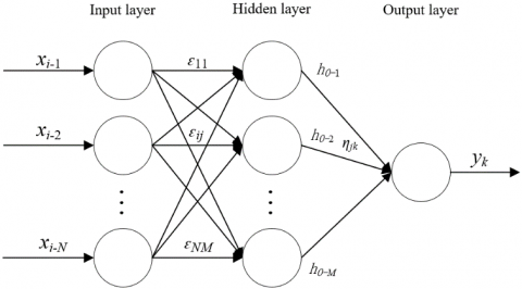
To make reasonable prediction of CIR risk propagation paths, this paper creates a multilayer feedforward NN with error backpropagation called the BPNN. The BPNN generally contain one input layer, n hidden layers, and one output layer. Assuming that only one predicted path is outputted, then the BPNN can be simplified as the multi-input, single-output network with only one hidden layer in Figure 2. Taking the TA(t), AE(t), and SR(t) values of the risk propagation model in Section 3 and the real-time changes of αab(t), βab(t), γab(t), p1(a, t), and p2(a, t) of each node as the inputs of the BPNN, an input vector can be constructed as:
$x_{i}=\left(x_{i-1}, x_{i-2}, \ldots, x_{i-N}\right)^{T}$ (12)
where, i is the serial number of the reconstruction processes of process and value chains; N is the number of input layer nodes. The hidden layer input can be expressed as:
$h_{I-j}=\sum_{i=1}^{N} \varepsilon_{i j} x_{i}-\lambda_{j}$ (13)
where, ԑij is the connection weight between the i-th input layer node and the j-th hidden layer node; λj is the threshold of the j-th hidden layer node. Then, the hidden layer output can be expressed as:
$h_{O-j}=\frac{1}{1+e^{-h_{j}}}$ (14)
The input of the k-th output layer node can be expressed as:
$g_{k}=\sum_{j=1}^{M} \eta_{j k} h_{O-j}-\delta_{k}$ (15)
where, ηjk is the connection weight between the j-th hidden layer node and the k-th output layer node; δk is the threshold of the k-th output layer node. Thus, the output of the output layer can be calculated by:
$y_{k}=\frac{1}{1+e^{-g_{k}}}$ (16)
Figure 2. The structure of the BPNN
4.2 BPNN training algorithm
The BPNN designed to predict the CIR risk propagation path was trained in six steps:
Step 1. Randomly initialize the connecting weights ԑij and ηjk, and thresholds λj and δk in the interval of [-1, 1], and import the sample data into the network.
Step 2. Calculate the input hI-j and output hO-j of the hidden layer, as well as the input gk and output yk of the output layer, according to formulas (13) and (14).
Step 3. Describe the mean squared error (MSE) between the expected output ŷk and the actual output yk as:
$V_{t}=\frac{1}{2} \sum_{k=1}^{M} \varphi_{k}^{2}=\frac{1}{2} \sum_{k=1}^{M}\left(\hat{y}_{k}-y_{k}\right)^{2}$ (17)
Calculate the negative value of the partial derivative of Vt to gk by:
$R_{t-k}=-\frac{\partial V_{t}}{\partial g_{k}}=\varphi_{k} y_{k}\left(1-y_{k}\right)=\left(\hat{y}_{k}-y_{k}\right) y_{k}\left(1-y_{k}\right)$ (18)
Calculate the negative value of the partial derivative of Vt to hidden layer input gk by:
$E_{t-j}=-\frac{\partial V_{t}}{\partial h_{I-j}}=\left(\sum_{t=1}^{M} R_{t-k} \eta_{j k}\right) h_{O-j}\left(1-h_{O-j}\right)$ (19)
Step 4. Let n be the number of iterations, and τ1 and τ2 be the correction coefficients. Then, update ηjk and δk respectively by:
$\eta_{j k}(n+1)=\eta_{j k}(n)+\tau R_{t-k} h_{O-j}$ (20)
$\delta_{k}(n+1)=\delta_{k}(n)-\tau R_{t-k}$ (21)
Update ԑij and λj respectively by:
$\varepsilon_{i j}(n+1)=\varepsilon_{i j}(n)+\tau_{2} E_{t-j} x_{i}$ (22)
$\lambda_{j}(n+1)=\lambda_{j}(n)-\tau_{2} E_{t-j}$ (23)
Step 5. Randomly select the parameters of the risk propagation model for the next reconstruction cycle, and import them to the network. Return to Step 4 until all samples are trained.
Step 6. Perform a new round of training until Vt falls in the interval of [-γ, γ], where γ is the preset training accuracy.
Based on the data disclosed by a company in its CIR 2019, this section carries out experiments on the reconstruction of process and value chains. During the reconstruction, the cycles, number of risk carriers, and types of risk carriers were collected, grouped into sample data with month as the time unit, and used to build a risk propagation network.
Table 3 provides the Cronbach’s alphas of the tertiary indices under each criterion after reliability analysis on SPSS 21.0. It can be seen that the Cronbach’s alphas of the tertiary indices averaged at 0.7, indicating the tertiary indices have good overall reliability.
Table 3. The Cronbach’s alphas of the tertiary indices under each criterion
|
Index |
Cronbach’s alpha |
Index |
Cronbach’s alpha |
Index |
Cronbach’s alpha |
Index |
Cronbach’s alpha |
Index |
Cronbach’s alpha |
|
A111 |
0.830 |
A121 |
0.656 |
A141 |
0.756 |
A221 |
0.547 |
A311 |
0.691 |
|
A111 |
0.567 |
A131 |
0.669 |
A141 |
0.746 |
A221 |
0.856 |
A311 |
0.901 |
|
A111 |
0.574 |
A131 |
0.745 |
A141 |
0.742 |
A221 |
0.641 |
A311 |
0.785 |
|
A111 |
0.412 |
A131 |
0.751 |
A141 |
0.845 |
A221 |
0.875 |
|
|
|
A121 |
0.689 |
A131 |
0.655 |
A211 |
0.941 |
A221 |
0.745 |
|
|
|
A121 |
0.745 |
A131 |
0.698 |
A211 |
0.679 |
A221 |
0.756 |
|
|
|
A121 |
0.874 |
A131 |
0.877 |
A211 |
0.697 |
A311 |
0.814 |
|
|
|
A121 |
0.745 |
A141 |
4.33 |
A211 |
0.845 |
A311 |
0.615 |
|
|
|
No. of reconstruction process |
Scale of CIR core subjects |
Degree of correlation between risk carriers |
C |
ωab |
α0 |
β0 |
Mean risk propagation probability |
Mean state recovery probability |
|
1 |
0.16 |
0.54 |
29 |
5 |
0.19 |
0.26 |
0.84 |
0.43 |
|
2 |
0.21 |
0.57 |
33 |
14 |
0.29 |
0.22 |
0.71 |
0.45 |
|
3 |
0.22 |
0.62 |
42 |
17 |
0.36 |
0.29 |
0.69 |
0.55 |
|
4 |
0.35 |
0.66 |
59 |
26 |
0.39 |
0.24 |
0.51 |
0.58 |
|
5 |
0.39 |
0.70 |
70 |
28 |
0.32 |
0.33 |
0.54 |
0.57 |
|
6 |
0.51 |
0.76 |
83 |
31 |
0.31 |
0.29 |
0.45 |
0.60 |
|
7 |
0.60 |
0.80 |
69 |
26 |
0.41 |
0.35 |
0.47 |
0.67 |
|
8 |
0.61 |
0.83 |
88 |
39 |
0.39 |
0.39 |
0.46 |
0.63 |
|
9 |
0.74 |
0.87 |
96 |
42 |
0.34 |
0.30 |
0.41 |
0.78 |
|
10 |
0.85 |
0.89 |
115 |
47 |
0.30 |
0.35 |
0.37 |
0.79 |
|
Mean |
0.46 |
0.72 |
68 |
28.5 |
0.33 |
0.30 |
0.34 |
0.83 |
Based on the hypotheses and parameter settings of our model, the reconstruction experiments were carried out, assuming that CIR risk propagation can be effectively controlled, that is, under the most ideal state out of the three possible states of risk propagation.
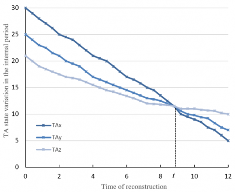
With the aid of Matlab, M functions Evo1.m, Evo2.m and Evo3.m and the M executable file Evorun.m were compiled for the results (8), (9), and (10) of CIR risk propagation in each period. The M functions were executed 60-80 times, and the results were combined and averaged. Figures 3, 4, and 5 display the results of CIR risk propagation in the internal, external, and final periods, respectively.
Figure 3. The TA state variation in the internal period
As shown in Figure 3, during the internal period, the TA(t) value decreased gently, and the CIR risk propagation reached the equilibrium at the intersection. Before the intersection, the reconstruction focuses on the prewarning of risk propagation; after the intersection, the reconstruction focuses on the restoration from the risk state. It can be seen that the keys of the reconstruction of the process and value chains lie in the reconstruction of the risk propagation prewarning module and risk state restoration module. During the reconstruction of risk propagation prewarning module, the risk flow direction and correlation between risk carriers directly bear on the risk control effect.
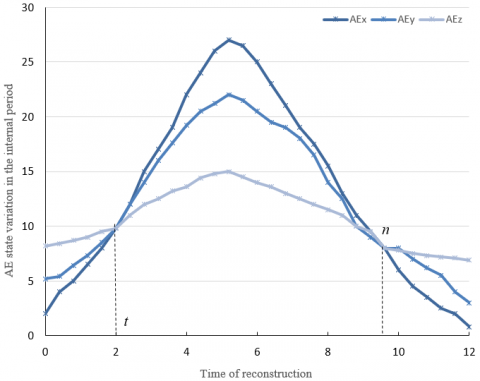
As shown in Figure 4, during the external period, the AE state exhibited as a parabolic curve. The left intersection is the critical point, at which risk propagation occurred between two risk carriers; the right intersection is the critical point, at which the risk diffusion changed into risk convergence. The left intersection was slightly higher than the right intersection. This means the overall safety of the CIR increases rapidly through the reconstruction cycle.
Figure 4. The AE state variation in the internal period
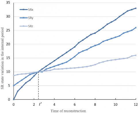
Figure 5. The SR state variation in the internal period
As shown in Figure 5, during the final period, the intersection is the critical point, at which the risk propagation between two risk carriers gradually stabilized and returned to the normal state. Before the intersection, the CIR was highly risky; after the intersection, the CIR risks were under control, i.e., the CIR was slightly safe. At the beginning of the final period, many nodes needed to be restored in the risk propagation network, and the recovery rate was rather slow. As more and more nodes were restored, the reconstruction process was simplified, and the node recovery gradually picked up speed. This means the CIR risk propagation has relatively high fluidity.
In addition, Figures 3-5 confirm the following finding from Table 4: when the CIR risk propagation is effectively controlled, the mean risk propagation probability of all risk carriers is on the decline, while the mean state recovery probability is on the rise.
The next task is to verify the prediction effect of our BPNN on CIR risk propagation path. For this purpose, 200 sets of TA(t), AE(t), and SR(t) of CIR risk propagation model and the αab(t), βab(t), γab(t), p1(a, t), and p2(a, t) values of each node were imported to the BPNN. Only one node output, which falls in [-1, 1], was allowed on the output layer, representing the overall evaluation result on the reconstruction and control effect of CIR risk propagation path.
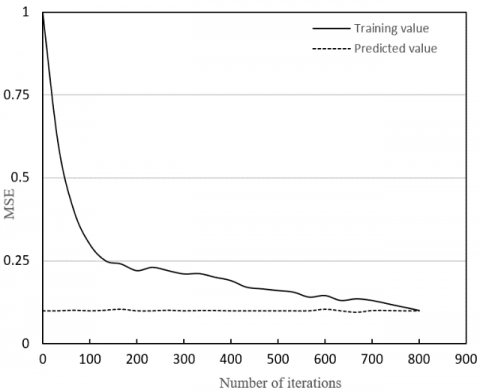
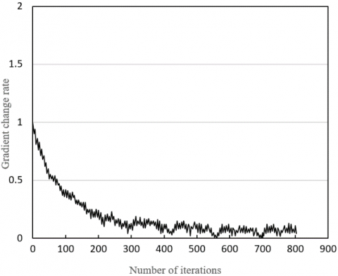
The BPNN was established on Matlab, including 48 input layer nodes, 24 hidden layer nodes, and 1 output layer node. As shown in Figures 6-8, the BPNN entered the convergence state and reach the preset training accuracy of 10-6, after 800 trainings. Besides, the BPNN predicted the CIR risk propagation path fairly accurately.
Figure 6. The MSE of prediction results
Figure 7. The simulated results on correlation gradient
Figure 8. The simulation results on prediction errors
This paper mainly presents an CIR risk propagation model based on the FNN. Firstly, an CIR safety EIS was created, and each of its index was subject to reliability analysis and weight calculation. Then, an FCE was carried out on the entire EIS. Through experiments, the Cronbach’s alphas of the secondary and tertiary indices under each criterion were obtained, after SPSS reliability analysis. Based on the evaluation results, the hypotheses and modes of risk propagation were summarized, creating the CIR risk propagation model. Several experiments were conducted on CIR risk propagation to disclose the variations of TA(t), AE(t), and SR(t) in different periods of the reconstruction process. The observed results confirm that the proposed model becomes increasingly safe through the reconstruction. Finally, a BPNN was constructed to predict the risk propagation path of the proposed model. Experimental results demonstrate that the BPNN can converge within the preset number of iterations, and make accurate predictions of CIR risk propagation path.
The Paper is supported by Fujian Social Science Fund Project: Research on Risk Ripple Effect and Crisis Management of Corporate Internet Reporting Based on SAR Framework (Grant No.: FJ2017C015).
[1] Stergiaki, E., Vazakidis, A., Stavropoulos, A. (2015). Development and evaluation of a prototype web XBRL-enabled financial platform for the generation and presentation of financial statements according to IFRS. International Journal of Accounting and Taxation, 31: 74-101. https://doi.org/10.15640/ijat.v3n1a5
[2] Martić, V. (2015). Application of XBRL-A in the function of improvement of quality of financial reporting in montenegro. Facta Universitatis-Economics and Organization, 12(4): 279-295.
[3] Skorupski, J. (2016). The simulation-fuzzy method of assessing the risk of air traffic accidents using the fuzzy risk matrix. Safety Science, 88: 76-87. https://doi.org/10.1016/j.ssci.2016.04.025
[4] Blankespoor, E., Miller, B.P., White, H.D. (2014). Initial evidence on the market impact of the XBRL mandate. Review of Accounting Studies, 19(4): 1468-1503. https://doi.org/10.1007/s11142-013-9273-4
[5] Efendi, J., Park, J.D., Smith, L.M. (2014). Do XBRL filings enhance informational efficiency? Early evidence from post-earnings announcement drift. Journal of Business Research, 67(6): 1099-1105. https://doi.org/10.1016/j.jbusres.2013.05.051
[6] Dijcks, J.P. (2012). Oracle: Big data for the enterprise. Oracle white paper, 16.
[7] Vasarhelyi, M.A., Chan, D.Y., Krahel, J.P. (2012). Consequences of XBRL standardization on financial statement data. Journal of Information Systems, 26(1): 155-167. https://doi.org/10.2308/isys-10258
[8] Janssen, M., van Veenstra, A.F., Van Der Voort, H. (2013). Management and failure of large transformation projects: Factors affecting user adoption. In International Working Conference on Transfer and Diffusion of IT, pp. 121-135. https://doi.org/10.1007/978-3-642-38862-0_8
[9] Harris, T.S., Morsfield, S.G. (2012). An evaluation of the current state and future of XBRL and interactive data for investors and analysts. https://doi.org/10.7916/D8CJ8NV2
[10] Alles, M., Piechocki, M. (2012). Will XBRL improve corporate governance? A framework for enhancing governance decision making using interactive data. International Journal of Accounting Information Systems, 13(2): 91-108. https://doi.org/10.1016/j.accinf.2010.09.008
[11] Seele, P. (2016). Digitally unified reporting: how XBRL-based real-time transparency helps in combining integrated sustainability reporting and performance control. Journal of Cleaner Production, 136: 65-77. https://doi.org/10.1016/j.jclepro.2016.01.102
[12] Kaya, D., Pronobis, P. (2016). The benefits of structured data across the information supply chain: Initial evidence on XBRL adoption and loan contracting of private firms. Journal of Accounting and Public Policy, 35(4): 417-436. https://doi.org/10.1016/j.jaccpubpol.2016.04.003
[13] Santos, I., Castro, E., Velasco, M. (2016). XBRL formula specification in the multidimensional data model. Information Systems, 57: 20-37. https://doi.org/10.1016/j.is.2015.11.001
[14] Lowe, A., Locke, J., Lymer, A. (2012). The SEC's retail investor 2.0: Interactive data and the rise of calculative accountability. Critical Perspectives on Accounting, 23(3): 183-200. https://doi.org/10.1016/j.cpa.2011.12.004
[15] Chen, B. (2019). Financial Market Reform in China: Progress, Problems, and Prospects. Routledge, ISBN: 0813336198
[16] Tsantekidis, A., Passalis, N., Tefas, A., Kanniainen, J., Gabbouj, M., Iosifidis, A. (2017). Forecasting stock prices from the limit order book using convolutional neural networks. In 2017 IEEE 19th Conference on Business Informatics (CBI), pp. 7-12. https://doi.org/10.1109/CBI.2017.23
[17] Breuel, T.M. (2017). High performance text recognition using a hybrid convolutional-LSTM implementation. In 2017 14th IAPR International Conference on Document Analysis and Recognition (ICDAR), Kyoto, pp. 11-16. https://doi.org/10.1109/ICDAR.2017.12
[18] Schmidhuber, J. (2015). Deep learning in neural networks: An overview. Neural Networks, 61: 85-117. https://doi.org/10.1016/j.neunet.2014.09.003
[19] Ribas, J.R., Arce, M.E., Sohler, F.A., Suárez-García, A. (2019). Data and calculation approach of the fuzzy AHP risk assessment of a large hydroelectric project. Data in Brief, 25: 104294. https://doi.org/10.1016/j.dib.2019.104294
[20] Negnevitsky, M., Nguyen, D.H., Piekutowski, M. (2014). Risk assessment for power system operation planning with high wind power penetration. IEEE Transactions on Power Systems, 30(3): 1359-1368. https://doi.org/10.1109/TPWRS.2014.2339358
[21] Centonze, P., Kim, D.Y., Kim, S. (2019). Security and privacy frameworks for access control big data systems. Comput. Mater. Continua, 59(2): 361-374. https://doi.org/10.32604/cmc.2019.06223
[22] Dineshreddy, V., Gangadharan, G.R. (2016). Towards an “Internet of Things” framework for financial services sector. In 2016 3rd International Conference on Recent Advances in Information Technology (RAIT), pp. 177-181. https://doi.org/10.1109/RAIT.2016.7507897
[23] Murjadi, M.D., Rustam, Z. (2018, December). Fuzzy support vector machines based on adaptive particle swarm optimization for credit risk analysis. In J. Phys., Conf. Ser., 1108(1): 1-6. https://doi.org/10.1088/1742-6596/1108/1/012052
[24] Cakra, Y.E., Trisedya, B.D. (2015). Stock price prediction using linear regression based on sentiment analysis. In 2015 International Conference on Advanced Computer Science and Information Systems (ICACSIS), pp. 147-154. https://doi.org/10.1109/ICACSIS.2015.7415179
[25] Shan, Y.G., Troshani, I., Richardson, G. (2015). An empirical comparison of the effect of XBRL on audit fees in the US and Japan. Journal of Contemporary Accounting & Economics, 11(2): 89-103. https://doi.org/10.1016/j.jcae.2015.01.001