Santhosh Kumar Veeramalla* | Venkata Krishna Hanumantha Rao Talari
OPEN ACCESS
The localization of neural sources is a crucial issue in medical, scientific and technical applications. However, the dipole sources in the brain may vary in nature and change constantly with time, adding to the difficulty of source localization. In this paper, the dynamic neural sources in the brain are simulated by sequential Monte-Carlo (MC) method, based on electroencephalography (EEG) data. Firstly, the EEG data were considered as a state space model. Considering the nonlinearity of the EEG data, the sequential M-C method was introduced as a particle filter, and the Metropolis-Hastings (M-H) resampling was employed to alleviate the particle impoverishment of general particle filter. The accuracy of our method in source localization was verified through two experiments, using both synthetic and real data. The research results shed important new light on the research of brain neurology.
electroencephalography (EEG), particle filter, source localization, Metropolis-Hastings (M-H) resampling
ELECTROENCEPHALOGRAPHY (EEG) is the non-invasive method of electrical activity recording or monitoring in the brain. EEG is used for visualizing and evaluation of the brain activity that are involved in how brain functions i.e. learning, memory, and emotions, or in neurological disorders such as autism, epilepsy and Parkinson's disease [1-3]. Localization of the neural sources using EEG, which are recorded from the scalp is broadly used to make appraisals of the areas of origins of the electrical movement in the cerebrum. Such data can be extremely valuable for both research and clinical applications. For instance, in clinical applications, exact data about the area of an epileptic seizure in the cerebrum can be utilized to design medical procedure for its expulsion. Moreover, data about the areas of the cerebrum that produce different signals can give important research data about the working of the cerebrum [4].
The location and distribution of current sources responsible for electrical activity in the brain based on the potentials of the electrodes is an important problem in the EEG. It is called the brain source position or the inverse EEG problem, given that data (potentials) are provided and the model needs to be built on the data that is available. The key results of EEG are the positions of source and the curses of neuronal activity found in the EEG field distribution. Nevertheless, several sources collections can produce exactly the same EEG field distribution. Brain activity localization dependent on EEG data requires a strongly ill-posed inverse problem to be resolved [5]. There have been a number of strategies to solve the reverse EEG problem in order to classify and recreate the origins of brain activity [6, 7].
A traditional EEG source model is a collection of equivalent current dipoles (ECD) which assume that a focal neuronal movement can be represented by one or more dipoles. This approach includes the multiple signal classification [8] and multi dipole modelling [9]. The dipole model's capacity to accurately identify neuronal reactions is nonetheless limited, given that 1) extended sources with ECD difficult to model and 2) the number of dipole is difficult to predict accurately. The other type of source reconstruction methods is dSPM [10], MNE [11], sLORETA [12]. For these approaches the source region (brain volume or cortex) is divided into a grid comprising many (normally thousands of) dipoles. Another form of methodology focused on point estimates, aimed at integrating sufficient knowledge prior to providing robust, accurate solutions, has been enhanced instead of declining through state space models [13, 14] and Markov Chain Monte Carlo [15]. Practical use can be performed efficiently and conveniently from the source position in a number of fields such as preoperative assessment and epilepsy.
Sequential Monte Carlo procedures are used to assess the present neural sources in the cerebrum that best suitable for the EEG measurement. Source localization can be implemented by discovering the scalp electric voltages that will come from the dipoles presented in the head. This part is called a forward problem, this can be calculated once relying upon the methodology utilized in the inverse problem. At that point, by thinking about the EEG information, it tends to be utilized to work back and estimate the neural sources which generate the EEG information is called the inverse problem [16].
Source localization of neural sources is a method that recreates the sources of electrical streams inside the cerebrum that offer to measured potentials on the head. In this paper, we will focus on locating neural sources from EEG data, which is an ill-posed issue. At a certain stage in time (i.e., the static case) [17], most attempts to take care of the inverse problem relied on scalp potentials. But in nature, the neural movement is dynamic. Subsequently, efforts were made in addressing the inverse problem to consider these components. This should be feasible by selecting appropriate strong models (which have distinctive arrangement requirements) [18].
Specifically, such ill-posedness infers that the neural design clarifying the estimations isn't one of a kind (there is a boundless number of neural current distributions delivering the similar dataset) and this specialized trouble has enlivened the reception of a wide range of methodologies for the determination of the ideal neural source localization from the unbounded arrangement of possible solutions [19].
Recently, Bayesian techniques have turned out to be a possible solution to the inverse problems due to an increase in the accessible computational power. In this article, we present a Bayesian filtering approach for the estimation of EEG dynamic sources. We take no hypotheses into account in this approach. Specifically, Monte Carlo techniques have been used in the EEG inverse problem situation. These strategies are used for an unidentified number of current dipoles to approximate posterior distribution. The basic idea of the Monte Carlo strategies is to approximate an integral use of a weighted particle system based on the distribution of probability. In the Bayesian methodology to deal with inverse issues, the goal is to compute and advantageously outline the posterior distribution, i.e., the conditional distribution of the unidentified given the deliberate information. In this article, we examine particle filters for the location of EEG dipole source where the amount of the dipole is unknown and time variant. We used this approach on synthetic data and here we showed that the source structure naturally could be assessed, as the reconstruction of the source is an ill-posed inverse problem and the reconstructed sources are not unique. In addition, we have used real EEG data to locate the unknown number of sources. They take the EEG readings as random variables in the inverse problem and the solution to the localization issue is to determine the feature of the posterior probability density of the unknown variables acquired by the theory of Bayes. Bayesian approaches use the entire time series as measurement information on a regular basis and these Bayesian methods can be regarded as methods that address the dynamic source localization issue [20].
The sequential Monte Carlo particle filter uses the Sequential Importance Sampling to approximate the subsequent state distribution at each moment. The particle filter utilizes an arrangement of particles to sample the state-space of the framework. These particles are then weighted using the measurement model to give a measure of the state posterior density. It can demonstrate that the estimation focalizes, in the mean-square error, to the true posterior density of the state. In any PF algorithm, there are three steps namely particle generation, weight calculation, and resampling. The first stage is the generation of particles and in the second stage assigns the weights. Lastly, resampling replaces the combination of both particles and weights with another set [21, 22].
The Bayesian methods basically track the probability distribution of the dipole parameters in time and the non-linear dependency on the dipole parameters of the data and the need for an estimate of the dipole number are the main problems. The main benefits of the Bayesian approaches are 1) the approach towards multiple dipole modeling is very general because it specifically allows the number of dipoles to vary in time and dynamically provides the resulting chance for the numbers of sources; (ii) it can be used in real time, because data is processed in sequentially and not in totality. The particle filter is used because of its dynamic nature to reconstruct different sources.
Particle filter performs very efficiently in the assessment of nonlinear and non-Gaussian dynamic system parameters. However, in computational terms, the particle filter algorithm is iterative and complicated. We will evaluate bottlenecks from current particle filter algorithms in this article and suggest a new strategy integrating particle filter with Metropolis-Hastings resampling algorithm. The neural activity is modelled as a stochastic process and the neural sources are tracked using the particle filter. This article presents a localization technique for EEG sources that uses the resampling algorithm Metropolis-Hastings to solve an inverse problem with the particle filter. This article proposes a new approach to reduce the PF computational complexity and improve the root mean-squared error (RMSE) estimates of the multi dipole localization problem. Results make it more effective to detect dipole sources when the algorithm holds an acceptable measurement value and seeks useful applications for epileptic patient information that predict the onset of dipole, keeping sufficient computational costs. The main objective of this article is to extract the 3-D source positions of the brain from the given EEG information. This can be used for clinical experiments or research i.e. it can be useful for localizing the epilepsy seizure sources etc.
The rest of the article is as follows, in section 2 we have described the inverse EEG problem. Section 3 introduces the particle filter and we describe the Metropolis-Hastings particle filter resampling algorithm and section 4 contains our results and a short discussion about main development work. Finally, Section 5 contains the final comments and bibliography.
In electrophysiology, the main issue is to predict the place of source from the measured EEG information, the inverse issue [23, 24]. To find the solution to the inverse problem, a model will be given to map the sources in the brain to the recorded data. Subsequently, the inverse problem is used by source localization with minimal error to find genuine useful functional tomography. Regardless, the standard test facing such an issue is that the estimates do not contain sufficient information about the sources that make the issue, not first-rate, and a perfect tomography cannot exist along these lines. The purpose of a test is to allow comparable external electromagnetic fields to be generated by differing internal source structures and to assess precisely these fields in a large and low number of areas [23].
In the cerebral cortex, which is the external surface of the brain, 10 billion neurons are included. Within this 1.5-4.5-mm thick piece of the brain the most observed scalp activity is produced. A synchronous synaptic reconstitution of a wide range of neurons leads to the symmetrical source of a dipolar current from which cortical surface appears [25]. Conscious EEG in distinct anode positions is the ultimate cause of this current.
After dealing with the inverse issue, one can use such a model to make an estimate of the EEG measurements from the decided dipoles. This is referred to as the forward issue. EEG inverse issue is about finding and limiting the source behind the deliberate electrical activity, which is ultimately fundamental and disease treatment. Precision in the construction and lighting of the model is essential for these cases. To discover the dipoles that best fit the observed data, we apply the inverse model. This inverse model's plan gives the locations of each dipole source.
Computation of the scalp potential requires a particular source demonstrate that must be understood numerically. In case the model relies upon probable head shapes, the computation might be a positive test. Scientific measures exist, at the same time, for efficient geometries, for example, while the head is expected to include an arrangement of nested concentric spheres relates to cerebrum, skull, and scalp. Those models are mechanically utilized as a part of most extreme clinical and studies bundles to EEG source localization.
Consider that N dipoles in cerebrum exhibits electrical activity. To evaluate such kind of activity the multi-channel EEG data can be used with $z _ { t } \in \Re$ from $n _ { s }$ number of sensors at a given time t, the forward EEG model is given by
$z _ { t } = L \left( x _ { t } \right) s _ { t } + v _ { t }$ (1)
The Eq. (1) refers to the moments of the dipole, the positions of the neural sources to the data recorded. S (t) is the vector of moments that contains moments of the dipole in three directions. Moments are equal to the number of time sample of the deliberate signals in the x, y and z directions of length that we are trying to model. The lead field matrix $L \left( x _ { t } \right)$ maps the dipole moments to the electrical potential of the scalp in a specified electrode position; and the dipole moments are measured by the volume of the matrix. vt,the noise measurement matrix. The model parameters are at every point in time based on the dipole quantity, the dipole time and the matrix for the lead field [26].
The Eq. (1) can be taken as a measurement equation, and for the state equation since it is unknown as to how the states evolve in the brain source localization problem,
$x _ { t } = x _ { t - 1 } + u _ { t }$ (2)
The above two Eqns. (1) and (2) can be considered as measurement or observation equation and state equation. From this, the EEG can be modeled as a state space model. To evaluate the dynamic parameters, i.e. location (x, y, and z-direction) in the cerebrum we use particle filter by considering the measured signal $z _ { t }$ at time $t$.
This part gives a brief idea about the particle filters. The nonlinear non-Gaussian system's state-space model [14] is given by:
$x _ { t } = f \left( x _ { t - 1 } \right) + u _ { t }$ (3)
$z _ { t } = h \left( x _ { t } \right) + v _ { t }$ (4)
where, $x _ { t }$ and $z _ { t }$ are respectively the state and measurement vectors, $f$ and $h$ are nonlinear functions of $x _ { t - 1 }$ and $z _ { t } , u _ { t }$ and $v _ { t }$ are the process noise and measurement noise while $t$ is the time index. It is assumed that the process and measurement noise is white noise, with the known functions of probability density and mutually independent. At time $t , z _ { t }$ can be represented as the EEG observations, and $h ( . )$ can be treated as a lead field matrix.
The main goal of particle filtering is to recurrently estimate the state $x _ { t }$ from the measurement $z _ { t } .$ The estimate of the unknown state $x _ { t }$ in Bayesian methods is based on the sequence of all $z _ { 1: t } = \left\{ z _ { 1 } , \ldots . . z _ { t } \right\}$ measurements up to time $t .$ The density function of the posterior probability is defined as $p \left( x _ { t } | z _ { 1: t } \right) .$ This subsequent distribution can be obtained recursively by using the density function prediction and update.
$p \left( x _ { t } | z _ { 1: t - 1 } \right) = \int p \left( x _ { t } | x _ { t - 1 } \right) p \left( x _ { t - 1 } | z _ { 1: t - 1 } \right) d x _ { t - 1 }$ (5)
The Eq. ( 5 ) can be used to estimate the prior pdf of the states at time $t .$ If the measurement is available at the time $t$ then the prior pdf in the Eq. (5) can be updated using Bayes rule.
$p \left( x _ { t } | z _ { 1: t } \right) = \frac { p \left( z _ { t } | x _ { t } \right) p \left( x _ { t } | z _ { 1: t - 1 } \right) } { p \left( z _ { t } | z _ { 1: t - 1 } \right) }$ (6)
The particle filter is used to discover the distribution function of the posterior likelihood provided in Eqns. (5) and (6) by random sampling or by producing particles. The following steps can be summarized as the standard particle filter algorithm: Particle producing, weight updating and resampling particles.
Generating a $N$ number of random particles $x ^ { ( i ) }$ is drawn from the importance density function $q \left( x _ { t } | x ^ { ( i ) } t - 1 , z _ { 1: t } \right)$ along with their weights $w ^ { ( i ) } t$ at time $t ,$ where $i = 1,2 , \ldots . N .$
The posterior density is given as $p \left( x _ { t } | z _ { 1: } \right) \approx$ $\sum _ { i = 1 } ^ { N } w ^ { ( i ) } t \delta \left( x _ { t } - x ^ { ( i ) } \right)$ where $\delta ( \cdot )$ is a Dirac delta function. The weights of the particles can be calculated as $w ^ { ( i ) } t \propto$ $w ^ { ( i ) } t - 1 \frac { p \left( z _ { t } | x ^ { ( i ) } t \right) p \left( x ^ { ( i ) } t \right) _ { t - 1 } \left( t ^ { ( i ) } t - 1 \right) } { q \left( x ^ { ( i ) } t | x ^ { ( i ) } t - 1 ^ { ( i ) } t _ { 1: t } \right) } .$ The sum of all weights should be equal to $1 .$
The serious problem with this particle filter is that after a certain number of iterations there is a weight degeneration problem. Weight degeneration means that only a small number of particles weigh one while the remaining particles weigh insignificantly. The distribution function of the posterior likelihood is not correct in this case. The particle filter must be resampled to avoid this problem.
The principal idea of the resampling is to re-sample the posterior probability density function of new particles. Resampling focuses mainly on large particles of weight and eliminates small particles of weight. In the resampling technique, small particles are dispensed, and enormous particles of weight are considered to influence the calculation of the appropriation of the priori [27]. The small weight particles have no responsibility at this stage to estimate the condition. It refers to the concept of particle deficiency. A variety of researchers have put forward strategies for preventing the impoverishment of particles [28]. The most popular method of systematic resampling is to sample one particle weight only from $\left( 0 , \frac { 1 } { N } \right)$ and to use the first particle to generate further particle weights.
$w _ { t } ^ { ( i ) } \sim U \left( 0 , \frac { 1 } { N } \right)$
$w _ { t } ^ { ( i ) } = w _ { t } ^ { ( 1 ) } + \frac { i - 1 } { N } , \quad i = 2,3 , \ldots \ldots N$ (7)
The systematic resampling is the bottleneck for the hardware implementation of particle filter [29, 30]. There are no information conditions for particle propagation and weight estimation, they can be effectively pipelined. Nonetheless, rigorous research includes data on all uniform weights which makes it difficult to perform with different steps. We propose another filtration technique that uses the Metropolis-Hastings resampling. As shown, this procedure gives the particle filter a systematic resampling equivalent estimation output.
We use the technique of Metropolis-Hastings (MH) to resample particle filters to overcome the problem caused by systematic resampling. MH Resampling begins when the principal weight of the particle is reachable [31]. The resampling of MH in specific does not involve each of the particles as a result of the creation of the chain of Markov in which the present state $x ^ { ( i ) }$ t depends exclusively on a previous state $x ^ { ( i ) } t - 1$ [32]. The MH calculation is
specifically able to extract particles from a probability function $p \left( x _ { t } \right)$ given a proposal importance probability density function $q \left( x _ { t } \right) .$ The fresh sample will then be adopted adopted or refused depending on the acceptability proportion in Eq. (8).
$r \left( x ^ { n } , x ^ { \prime } \right) = \min \left\{ 1 , \frac { p \left( x ^ { \prime } \right) q \left( x ^ { n } | x ^ { \prime } \right) } { p \left( x ^ { n } \right) q \left( x ^ { n } | x ^ { \prime } \right) } \right\}$ (8)
where, $x ^ { \prime } \sim q \left( \cdot | x ^ { n } \right)$ and $q ( . )$ is the desired importance density. Generate a uniform random variable $u \sim U ( 0,1 ) .$ The particles $x ^ { ( i ) } t$ are resampled using $\mathrm { MH } ;$ therefore high-weight particles are replaced and low-weight particles are disposed of. The rest of the particles therefore speak more precisely to the posterior probability density function, leading to improved execution.
We use the proposed PF algorithm to track the unknown number of neural sources using both synthetic and real EEG data to demonstrate tracking performance.
4.1 Synthetic data results
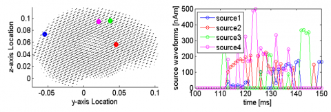
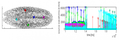
Our study with synthetic data [33], sampled at 256 Hz, corresponds to four neural sources which are uniformly constructed over and at angles of hemispheric head area. The results of RMSE execution are first shown through the use of synthetic data for the different dipole neural activity tracking. The information was obtained by embedding current dipoles and figuring the subsequent electric field into the concentrated sphere head model. Figure 1 shows the true source positions and source amplitudes across the specified time interval, Table 1 provides the true (original) dipole source positions. We run the particle filter with 20,000 sample points.
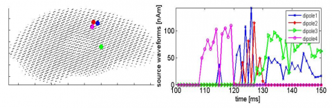
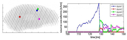
Figures 2 and 3 speak to the source areas of the synthetic data by using the particle filter with systematic and MH resampling methods respectively. The estimation execution as far as RMSE for both resampling cases is outlined in Table 2. 50 Monte Carlo runs were performed to get the RMSE. Here, we additionally incorporate RMSE of the Beamforming calculation [34] for examination. We can see that although systematic and MH resampling strategies both give sensible appraisals of the dipole sources, the MH resampling gauges the dipoles essentially with improved RMSE. Besides, the RMSE of the particle filter is also smaller than the other algorithms as specified in Table 3. The distance RMSE between true source and estimated dipole for the proposed method is 3.82 mm. The simulations with synthetic data show the proficiency of the proposed strategy for confining and remaking exceptionally cerebrum sources from synthetic data.
Figure 1. True source positions and source amplitudes of the synthetic data
Table 1. True dipole positions in synthetic data
|
Dipole source |
Position (3-dimension) in cm |
||
|
X-axis |
Y-axis |
Z -axis |
|
|
source 1 |
−1.37 |
−5.43 |
7.34 |
|
source 2 |
3.74 |
4.54 |
5.66 |
|
source 3 |
−2.04 |
3.73 |
9.56 |
|
source 4 |
2.96 |
2.11 |
9.42 |
Figure 2. Estimated source positions using systematic resampling for the synthetic data
Figure 3. Estimated source positions using Metropolis-Hastings resampling for the synthetic data
Table 2. Average RMSE (in mm) of the 3-d position and computational time of resampling schemes
|
Sources |
Resampling method |
|
|
Systematic |
MH |
|
|
1 |
5.76 |
5.45 |
|
2 |
2.56 |
0.64 |
|
3 |
3.68 |
6.73 |
|
4 |
3.91 |
2.45 |
|
Average RMSE |
3.97 |
3.82 |
|
Computational time |
4.26s |
3.84s |
|
Approach |
No. of dipole sources |
RMSE |
|
MPF [35] |
2 |
6.1 |
|
RBPF [36] |
2 |
6.3 |
|
PF [20] |
4 |
5.4 |
|
Proposed method |
4 |
3.82 |
4.2 Real EEG data
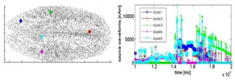
The main problem in evaluating the efficiency of EEG source localization algorithms in real settings is the unknown of actual EEG neural generators. In an experimental set of data taken from the Brainstorm EEG / Epilepsy [37] dataset, we apply the proposed particle filter. Data consist of 29-electrode EEG recordings of an epileptic subject (FP1, FP2, F3, F4, C3, C4, P3, P4, O1, O2, F7, F8, T7, T8, P7, P8, Fz, Cz, Pz, T1, T2, FC1, FC2, FC5, FC6, CP1, CP2, CP5, CP6) in accordance with the 10/20 International Framework. Note that we don't have a definite position of the neural sources of real information, so we can't deliver the RMSE of the area of the dipoles. Consequently, we took computational time as a proportion of contrasting the resampling plans is given in Table 4. It is observed that computational time is more for MH resampling, this is because of large datasets but based on the RMSE of the synthetic data we can say that MH resampling provides a good estimation of the neural sources. Figures 4 and 5 represent the estimated source positions and their amplitude waveforms of the real data using the particle filter with systematic and MH resampling correspondingly.
Table 4. Comparison of computational time in seconds between various resampling schemes
|
Resampling method |
Systematic |
Metropolis |
|
Computational time (sec) |
5020 |
7270 |
Figure 4. Estimated source positions using Systematic resampling for the real EEG information
Figure 5. Estimated source positions using Metropolis-Hastings resampling for the real EEG information
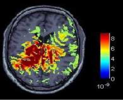
Figure 6. Estimated source positions with sLoreta for the real EEG information
We compare the estimated sources of the particle filter with the findings of sLoreta. Figure 6 shows the results of the sLoreta process. The particle filtering and sLoreta are given with similar sources. The findings are consistent with the real EEG estimates from previous physiological studies. The data from the focal epileptic patient in our dataset means that the origins can be in the temporal lobe of the brain. The results show that most origins are in the brain's temporal lobe.
4.3 Discussion
This article described a neural particle filter system based on the probabilistic fusion of several models of the dipolar source. Every model is defined as a dynamic system with the number of sources (every source model has a dipole with its current location and moment). The particle filter clearly differentiates the operation of each origin while multi dipole models take the time cycles given during the analysis process. In essence, the particle filter is a multi-target tracking algorithm that simultaneously reconstructs active dipoles and outperforms other reconstruction methods.
Importantly, this sLoreta method takes the input as a single point of time instead of a time series. In the same window, the source activations produced from a proposed particle filter are compared to those from the same signal pick. This approach is based on a distributed source model rather than a dipolar source model. sLoreta usually offers large maps with relatively strong sources and less disseminated maps with relatively low sources as the posterior likelihood of a strong source is high and vice versa. The estimates of sLoreta are shown in Figure 6. The colored region of the brain cortex is the scaled plot of sLoreta, and the colored bars to the right reflect the intensity of the inverse sLoreta solution. The methods of sLoreta and particle filtering differ greatly. The image produced by sLoreta represents the approximate intensity of the neural current, but the images created from the particle filter algorithm reflect a probability that a neural source exists at any given position. Nevertheless, sLoreta and particle filter methods appear to agree in a comfortable manner on the supposed cerebral position PF methods generate location estimates with time monitoring throughout the whole time window.
The EEG provides a good resolution for explaining neuronal activity as an imaging tool, but contributes to poor spatial resolution and which results in undesirable characteristics when the sources are located. Consequently various methods for solving the EEG Inverse problem are developed and explained by researchers. In addition, the effects of time correlations, position error and methodological mathematical relations are main parameters, as described above.
Sequential Monte Carlo Particle filter implementations of Bayesian filters used to map the density of probability of a time varying evolutionary process by a weighted set of particles. The conceptual significance of the use of particle filters includes the spatial and temporal characteristics of the neural sources behind them. We have shown the neural dynamic source localization with the unknown number of dipoles using the particle filter. In this paper, a Metropolis-Hastings procedure has been acquainted to alleviate the particle impoverishment issue experienced in the general particle filter. MH procedure is utilized to dispose of the little weight particles and acknowledge the large weight ones dependent on the acceptance ratio. In the interim, particle diversity can be improved to a huge degree. The accuracy of the proposed approach to source localization is validated from synthetic and real data. The results of these two experiments show that the particle filter with MH resampling is more accurate than the general particle filter. The result which determines the positions of brain activity due to focal epileptic information, is consistent with current knowledge about neuropsychology. The computational costs depend on the number of particles used and the amount of time samples used in the particle filter. Probably the most common approach is the particle filter. In the particle filter, research is still needed for the estimation of the solution from particles because when the source dipoles increase, the conditional mean is less effective.
|
$x _ { t }$ |
State vector |
|
$Z _ { t }$ |
Measurement vector |
|
$u _ { t }$ $v _ { t }$ |
Process noise Measurement noise |
|
$h ( . )$ $p \left( x _ { t } | z _ { 1: t } \right)$ $q ( . )$ w |
Leadfield matrix Posterior probability of $x _ { t }$ given $Z _ { 1: t }$ Importance density Weight of the particle |
[1] Stevens, M.C. (2009). The developmental cognitive neuroscience of functional connectivity. Brain and Cognition, 70(1): 1-12. http://dx.doi.org/10.1016/j.bandc.2008.12.009
[2] Belmonte, M.K., Allen, G., Beckel-Mitchener, A., Boulanger, L.M., Carper, R.A., Webb, S.J. (2004). Autism and abnormal development of brain connectivity. Journal of Neuroscience, 24(42): 9228-9231. http://dx.doi.org/10.1523/JNEUROSCI.3340-04.2004
[3] Uhlhaas, P.J., Singer, W. (2006). Neural synchrony in brain disorders: Relevance for cognitive dysfunctions and pathophysiology. Neuron, 52(1): 155-168. http://dx.doi.org/10.1016/j.neuron.2006.09.020
[4] De Munck, J.C., Van Dijk, B.W., Spekreijse, H.E.N.K. (1988). Mathematical dipoles are adequate to describe realistic generators of human brain activity. IEEE Transactions on Biomedical Engineering, 35(11): 960-966. http://dx.doi.org/10.1109/10.8677
[5] Sarvas, J. (1987). Basic mathematical and electromagnetic concepts of the biomagnetic inverse problem. Physics in Medicine & Biology, 32(1): 11. http://dx.doi.org/10.1088/0031-9155/32/1/004
[6] Baillet, S., Mosher, J.C., Leahy, R.M. (2001). Electromagnetic brain mapping. IEEE Signal Processing Magazine, 18(6): 14-30. http://dx.doi.org/10.1109/79.962275
[7] Michel, C.M., Murray, M.M., Lantz, G., Gonzalez, S., Spinelli, L., de Peralta, R.G. (2004). EEG source imaging. Clinical Neurophysiology, 115(10): 2195-2222. http://dx.doi.org/10.1016/j.clinph.2004.06.001
[8] Mosher, J.C., Lewis, P.S., Leahy, R.M. (1992). Multiple dipole modeling and localization from spatio-temporal MEG data. IEEE Transactions on Biomedical Engineering, 39(6): 541-557. http://dx.doi.org/10.1109/10.141192
[9] Huang, M., Aine, C.J., Supek, S., Best, E., Ranken, D., Flynn, E.R. (1998). Multi-start downhill simplex method for spatio-temporal source localization in magnetoencephalography. Electroencephalography and Clinical Neurophysiology/Evoked Potentials Section, 108(1): 32-44. http://dx.doi.org/10.1016/S0168-5597(97)00091-9
[10] Dale, A.M., Liu, A.K., Fischl, B.R., Buckner, R.L., Belliveau, J.W., Lewine, J.D., Halgren, E. (2000). Dynamic statistical parametric mapping: combining fMRI and MEG for high-resolution imaging of cortical activity. Neuron, 26(1): 55-67. http://dx.doi.org/10.1016/s0896-6273(00)81138-1
[11] Hämäläinen, M.S. (2005). MNE software user's guide. NMR Center, Mass General Hospital, Harvard University, 58: 59-75.
[12] Pascual-Marqui, R.D. (2002). Standardized low-resolution brain electromagnetic tomography (sLORETA): Technical details. Methods Find Exp Clin Pharmacol, 24(Suppl D): 5-12.
[13] Long, C.J., Purdon, P.L., Temereanca, S., Desai, N.U., Hamalainen, M., Brown, E.N. (2006). Large scale Kalman filtering solutions to the electrophysiological source localization problem-a MEG case study. 2006 International Conference of the IEEE Engineering in Medicine and Biology Society. IEEE. http://dx.doi.org/10.1109/IEMBS.2006.259537
[14] Sorrentino, A., Parkkonen, L., Pascarella, A., Campi, C., Piana, M. (2009). Dynamical MEG source modeling with multi‐target Bayesian filtering. Human Brain Mapping, 30(6): 1911-1921. http://dx.doi.org/10.1002/hbm.20786
[15] Jun, S.C., George, J.S., Paré-Blagoev, J., Plis, S.M., Ranken, D.M., Schmidt, D.M., Wood, C.C. (2005). Spatiotemporal Bayesian inference dipole analysis for MEG neuroimaging data. NeuroImage, 28(1): 84-98. http://dx.doi.org/10.1016/j.neuroimage.2005.06.003
[16] Hallez, H., Vanrumste, B., Grech, R., Muscat, J., De Clercq, W., Vergult, A., D'Asseler, Y., Camilleri, K.P., Fabri, S.G., Van Huffel, S., Lemahieu, I. (2007). Review on solving the forward problem in EEG source analysis. Journal of Neuroengineering and Rehabilitation, 4(1): 46. http://dx.doi.org/10.1186/1743-0003-4-46
[17] Grech, R., Cassar, T., Muscat, J., Camilleri, K.P., Fabri, S.G., Zervakis, M., Xanthopoulos, P., Sakkalis, V., Vanrumste, B. (2008). Review on solving the inverse problem in EEG source analysis. Journal of Neuroengineering and Rehabilitation, 5(1): 25. http://dx.doi.org/10.1186/1743-0003-5-25
[18] Yamashita, O., Galka, A., Ozaki, T., Biscay, R., Valdes-Sosa, P. (2004). Recursive penalized least squares solution for dynamical inverse problems of EEG generation. Human Brain Mapping, 21(4): 221-235. http://dx.doi.org/10.1002/hbm.20000
[19] Whittingstall, K., Stroink, G., Gates, L., Connolly, J.F., Finley, A. (2003). Effects of dipole position, orientation and noise on the accuracy of EEG source localization. Biomedical Engineering Online, 2(1): 14.
[20] Sorrentino, A., Parkkonen, L., Piana, M. (2007). Particle filters: A new method for reconstructing multiple current dipoles from MEG data. International Congress Series, 1300: 173-176. http://dx.doi.org/10.1016/j.ics.2007.02.026
[21] Li, T.C., Bolic, M., Djuric, P.M. (2015). Resampling methods for particle filtering: Classification, implementation, and strategies. IEEE Signal Processing Magazine, 32(3): 70-86. http://dx.doi.org/10.1109/MSP.2014.2330626
[22] Miodrag, B., Djurić, P.M., Hong, S.J. (2004). Resampling algorithms for particle filters: A computational complexity perspective. EURASIP Journal on Advances in Signal Processing, 15: 403686. https://doi.org/10.1155/S1110865704405149
[23] Pascual-Marqui, R.D. (1999). Review of methods for solving the EEG inverse problem. International Journal of Bioelectromagnetism, 1(1): 75-86.
[24] Ebersole, J.S., Pedley, T.A. (2003). Current Practice of Clinical Electroencephalography. Lippincott Williams & Wilkins.
[25] Zhukov, L., Weinstein, D., Johnson, C. (2000). Independent component analysis for EEG source localization. IEEE Engineering in Medicine and Biology Magazine, 19(3): 87-96. http://dx.doi.org/10.1109/51.844386
[26] Somersalo, E., Voutilainen, A., Kaipio, J.P. (2003). Non-stationary magnetoencephalography by Bayesian filtering of dipole models. Inverse Problems, 19(5): 1047. http://dx.doi.org/10.1088/0266-5611/19/5/304
[27] Khan, Z., Balch, T., Dellaert, F. (2004). An MCMC-based particle filter for tracking multiple interacting targets. European Conference on Computer Vision. Springer, Berlin, Heidelberg. http://dx.doi.org/10.1007/978-3-540-24673-2_23
[28] Rui, Y., Chen, Y.Q. (2001). Better proposal distributions: Object tracking using unscented particle filter. CVPR, (2).
[29] Athalye, A., Bolic, M., Hong, S., Djuric, P.M. (2004). Architectures and memory schemes for sampling and resampling in particle filters. 3rd IEEE Signal Processing Education Workshop. 2004 IEEE 11th Digital Signal Processing Workshop, 2004, Taos Ski Valley, NM, USA. http://dx.doi.org/10.1109/DSPWS.2004.1437918
[30] Athalye, A., Bolić, M., Hong, S., Djurić, P.M. (2005). Generic hardware architectures for sampling and resampling in particle filters. EURASIP Journal of Applied Signal Processing, 17: 2888-2902. http://dx.doi.org/10.1155/ASP.2005.2888
[31] Sankaranarayanan, A.C., Srivastava, A., Chellappa, R. (2008). Algorithmic and architectural optimizations for computationally efficient particle filtering. IEEE Transactions on Image Processing, 17(5): 737-748. http://dx.doi.org/10.1109/TIP.2008.920760
[32] Christian, R., Casella, G. (2013). Monte Carlo Statistical Methods. Springer Science & Business Media.
[33] Campi, C., Pascarella, A., Sorrentino, A., Piana, M. (2011). Highly automated dipole estimation (HADES). Computational Intelligence and Neuroscience, 2011, Article ID 982185. http://dx.doi.org/10.1155/2011/982185
[34] Groß, J., Kujala, J., Hämäläinen, M., Timmermann, L., Schnitzler, A., Salmelin, R. (2001). Dynamic imaging of coherent sources: Studying neural interactions in the human brain. Proceedings of the National Academy of Sciences, 98(2): 694-699. http://dx.doi.org/10.1073/pnas.98.2.694
[35] Miao, L., Zhang, J.J., Chakrabarti, C., Papandreou-Suppappola, A. (2012). Efficient Bayesian tracking of multiple sources of neural activity: Algorithms and real-time FPGA implementation. IEEE Transactions on Signal Processing, 61(3): 633-647. http://dx.doi.org/10.1109/TSP.2012.2226172
[36] Campi, C., Pascarella, A., Sorrentino, A., Piana, M. (2008). A Rao–Blackwellized particle filter for magnetoencephalography. Inverse Problems, 24(2): 025023. https://doi.org/10.1088/0266-5611/24/2/025023
[37] Tadel, F., Baillet, S., Mosher, J.C., Pantazis, D., Leahy, R.M. (2011). Brainstorm: a user-friendly application for MEG/EEG analysis. Computational Intelligence and Neuroscience, 2011. http://dx.doi.org/10.1155/2011/879716