Lu Bai* | Chenglie Du
OPEN ACCESS
This paper attempts to solve the 2D global path planning problem in a known environment. For this purpose, a smooth path planning method was designed for mobile robots based on dynamic feedback A* search algorithm and the improved ant colony optimization (ACO). Specifically, the ACO was improved from three aspects: optimizing the initial pheromone, improving evolutionary strategy and implementing dynamic closed-loop adjustment of parameters. The planned path was then smoothened by the cubic B-spline curve. The simulation results show our method converged to a shorter path in less time than the original ACO, and avoided the local optimum trap.
path planning, ant colony optimization (ACO), collision-free algorithm, B-spline curve
In the field of mobile robot, autonomous navigation [1-2] is the key technology of intelligent robot motion system. Whether a mobile robot can complete tasks with high quality depends on two factors, namely, reliable positioning and efficient path planning. Currently, it is a challenging issue to plan efficient paths and locate targets accurately in mobile robot navigation system.
So far, many achievements have been made in path planning and target positioning of mobile robots. However, there are still some problems with the existing methods. For example, robot positioning and environment map-making should be more accurate and stable, the path planning algorithm should satisfy the features and constraints of robot motion, and the paths should be planned more efficiently in a short time. Therefore, the path planning of mobile robots is selected as the object of this research.
Depending on the mastery of environmental information, the existing path planning methods for mobile robots mainly fall into two categories: the local path planning based on sensor environment, and the global path planning based on environmental information [3-4]. Local path planning aims to construct a collision-free path when part or all environmental information is unknown. The information of obstacles, including size, shape and location, needs to be updated in real time by the sensors on the mobile robot. Otherwise, it would be impossible to obtain the obstacle distribution in the surroundings.
In global path planning, the environmental information like the initial pose and target is already known, and the optimal collision-free path from the start node to the target node can be planned through repeated computations. The path quality should be evaluated against certain criteria, such as distance, time, smoothness or energy. Among them, distance and time are the most common criteria.
Skeleton-based search algorithm [5], heuristic search method [6] and intelligent optimization algorithm [7] are the leading techniques for global path planning of mobile robots.
Skeleton-based search algorithm relies on either visibility graph [8-9] or Voronoi diagram [10]. The visibility graph describes each obstacle of mobile robot with a convex polygon, treats each position of the robot as a node, and links up the start node S, target node G and the polygon vertices with edges. Thus, the path planning is to select the combination of edges with the shortest distance. Liu et al. [11] reduced the number of edges in the visibility graph based on the impacts of obstacles on path planning, and proved through simulation that the reduction makes the path planning algorithm more efficient. Faigl et al. [12] proposed two time-efficient methods for global path planning of robots. Kim et al. [13] proposed a fast, dynamic visibility graph to construct a simplified path map to circumvent the convex polygons (obstacles). Tsardoulias et al. [14] put forward a global path planning method based on visibility graph, which reduces the path length by 14% on average while maximizing the curvature plus its derivative and continuity. The Voronoi diagram is inspired by the Cartesian space partitioning in convex domain. Based on Voronoi diagram, the path planning algorithm can simplify complex spatial search into a path search in a weighted graph. Shao et al. [15] developed a local smooth path planning algorithm based on Voronoi diagram for mobile robots with vehicle motion features.
The heuristic search algorithm looks for the optimal path by the heuristic function, and estimates the distance between the current node and the target node. For example, the A* search algorithm, due to its simple principle, has been adopted widely for global path planning of 2D mobile robots. However, this heuristic search algorithm faces several problems: some planned nodes are redundant, and the inflection nodes of the planned path have a fixed attitude. To solve these problems, Yuan et al. [16] improved the A* search algorithm for indoor mobile robots, and successfully optimized the path in grid environment.
The intelligent optimization algorithm has many advantages in path planning, owing to the progress in modern control technology. Considering the features of terrain and landform, Akbarimajd et al. [17] proposed an offline robot path planner based on ant colony optimization (ACO) to find the ideal path between any points of a given terrain. Das et al. [18] developed an optimal path planning algorithm for mobile robots, drawing on gravity search algorithm and particle swarm optimization (PSO). Wang et al. [19] employed the ACO to search for the global optimal path for mobile robots based on raster map. Navarro et al. [20] designed a path planning method for mobile robots based on adaptive ACO in global static environment, aiming to speed up the convergence of the ACO and prevent the algorithm from falling into the local optimum trap. Oleiwi et al. [21] combined the ACO and the genetic algorithm (GA) into a hybrid global path planning algorithm for multi-objective optimization of mobile robots.
In the global path planning of mobile robots, the environment model mainly aims to describe the location of the mobile robot, obstacles, as well as initial and end points in the real environment. A good environment model enables the mobile robot to navigate autonomously with high accuracy and flexibility, and to plan the optimal, feasible path more efficiently.
In this paper, the raster map is selected to build the environment model and partition the workspace of the mobile robot. By this common method for map modelling, the environment is characterized with a binary raster array, and the robot workspace is meshed into a series of large grids, in the light of the size of the mobile robot. So far, the raster map has been successfully coupled with various algorithms for global path optimization, because it is simple, effective, and suitable for computer storage and data processing.
The raster map is essentially a mapping between the features of the actual environment space and the nodes of the abstract space. During the mapping process, the environment space is firstly transformed into a raster map. Then, the path-finding algorithm looks for the set of continuous nodes that make up the optimal path, and connect them with edges or arcs. Based on the raster map, the environment modeling can be implemented in three steps.
(1) Raster division
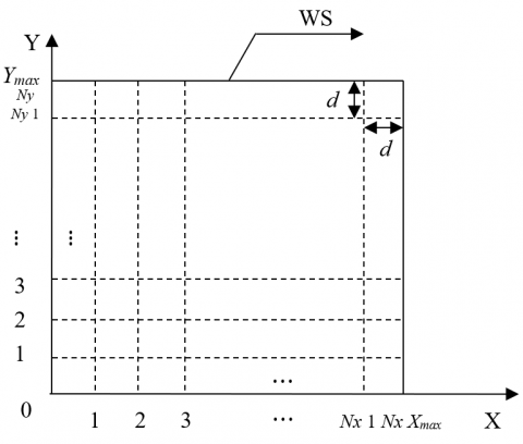
The 2D finite workspace of the mobile robot is shown in Figure 1, where WS is the workspace; Xmax and Ymax are the maximum value of the workspace on X and Y axes, respectively; d is the minimum step length of the robot. In this step, the workspace was divided by a set of lines with the length of d, creating $N_{x} \times N_{y}$ grids.
(2) Obstacle expansion
For convenience, the mobile robot was transformed into particles based on its size. Meanwhile, the obstacles in the environment were expanded in size.
(3) Construction of 2D raster array matrix
After obstacle expansion, the workspace was divided into two raster sets: the obstacle raster set OS and the free raster set FS. The corresponding value of the elements in the former set is 1, while that in the latter set is 0. Thus, the raster space can be expressed as:
$W S(\mathrm{i}, \mathrm{j})=\left\{\begin{array}{ll}{1} & {W S_{i j} \in O S} \\ {0} & {W S_{i j} \in F S}\end{array}\right.$ (1)
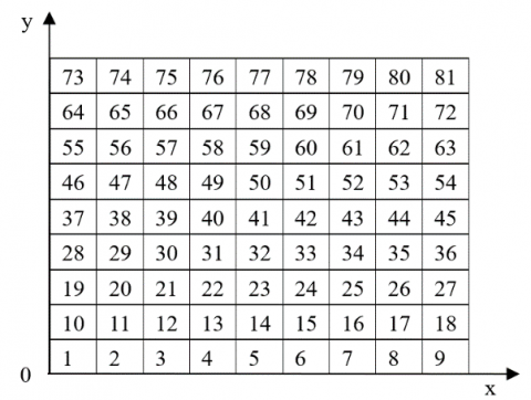
In raster environment, the order and position of a raster in the map are usually described with a serial number and coordinates, respectively. The serial number is unique to each raster because the grids were numbered from left to right and from bottom to top, starting from the lower left corner of the raster map. The relationship between raster coordinates and serial number is illustrated in Figure 2.
Figure 1. Raster division of the workspace
Figure 2. The relationship between raster coordinates and serial number
Based on the above relationship, the transformation can be expressed as:
$\left\{\begin{array}{l}{x_{i}=i \bmod N_{x}} \\ {y_{i}=i \text { int } N_{y}}\end{array}\right.$ (2)
where, mod is the exponentiation operation; int is the rounding operation.
To speed up the search of the ACO, a simplified A* algorithm was introduced to optimize the distribution and thus quality of the initial pheromone, making the initial search more targeted. In addition, the closed-loop feedback was adopted to adjust the parameters dynamically and adaptively, aiming to further enhance the adaptability and avoid the local optimum trap. Finally, the planned path was smoothened with cubic B-spline curve.
4.1 Improvement of initial pheromone
In the initial iteration of the ACO, most of the initial pheromones are distributed uniformly, due to the lack of the prior information on the whole graph. In other words, all paths have the same initial value of pheromone, denoted by a constant C. To speed up the initial search and reduce the number of iterations, the simplified A* algorithm and map information were introduced to optimize the initial pheromone distribution.
The A* algorithm [22], a classical heuristic search algorithm, is the most effective direct method to search for the shortest path in static environment. The evaluation function f(n) of the current node n can be expressed as:
$f(n)=s(n)+t(n)$ (3)
where, $s(n)$ is the actual cost to move from the current node n to the initial point $S\left(x_{s}, y_{s}\right)$; $t(n)$ is the evaluated cost to move from the current node n to the target node $G\left(x_{g}, y_{g}\right)$.
Taking the start node as the starting point of the search, the simplified A* algorithm selects collision-free nodes from the nodes connected to the start node, and adds them to the OPEN table based on the evaluation function of the current node. Then, the adjacent node with the minimum evaluated cost will be stored in the CLOSE table. After that, this node will be placed in the OPEN table and serve as the current node in the search of the next node. Similarly, the node with the minimum evaluated cost will be stored in the CLOSE table. The above steps are repeated until the end node appears in the OPEN table.
In this way, the optimal path can be found based on the evaluation function, and expressed by the nodes stored in the CLOSE table. Let Rb be the search path obtained based on the evaluation function f(n). Then, the initial value of the pheromone on the enhanced path can be described as:
$\tau\left(R_{b}\right)=k \times C,(k>1)$ (4)
4.2 Dynamic closed-loop adjustment of ACO parameters
The ACO’s ability to handle practical problems hinges directly on its parameters [23]. There are five parameters in the improved ACO, namely, the number of ants in the colony, m; the adjustment probability of the search space, $p_{0}$; the pheromone heuristic factor, $\alpha$; the visibility heuristic factor, $\beta$; the pheromone volatilization coefficient, $\rho$. The impacts of each parameter on path length are given in Table 1.
Table 1. Parameter analysis for path length
|
Parameter |
Environment 1 |
Environment 2 |
Scope |
||||
|
Shortest path value |
Longest path value |
Difference value |
Shortest path value |
Longest path value |
Difference value |
||
|
$\beta$ |
28.33 |
30.12 |
1.79 |
30.76 |
31.08 |
0.32 |
2-20 |
|
$\rho$ |
28.33 |
29.75 |
1.42 |
30.76 |
31.51 |
0.75 |
0.2-0.8 |
|
$p_{0}$ |
28.33 |
78.64 |
50.31 |
30.76 |
83.67 |
52.91 |
0.1-1 |
As shown in Table 1, $p_{0}$ is the main factor affecting path length, and was thus selected as the target of dynamic closed-loop adjustment. The adjustment formula of parameter $p_{0}$ can be expressed as:
$\left\{\begin{array}{ll}{q_{0}^{t+1}=q_{0}^{t} \times\left(1-\frac{\left(L_{b}^{t+1}-L_{b}^{t}\right)}{L_{b}^{t}}\right),} & {\text { if } L_{b}^{t+1} \neq L_{b}^{t}} \\ {q_{0}^{t+1}=q_{0}^{t},} & {\text { if } L_{b}^{t+1}=L_{b}^{t} \wedge \operatorname{num}\left(L_{b}^{t+1}=L_{b}^{t}\right)<N_{\text {max }}} \\ {q_{0}^{t+1}=\varepsilon q_{0}^{t},} & {\text { if } L_{b}^{t+1}=L_{b}^{t} \wedge \operatorname{mum}\left(L_{b}^{t+1}=L_{b}^{t}\right) \geq N_{\text {max }}}\end{array}\right.$ (5)
4.3 Path smoothing based on cubic B-spline curve
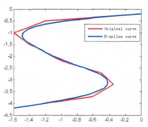
The path planned for mobile robot must be smooth enough for the robot to maneuver easily in actual environment. Since the ACO plans the path in the raster map, the output path is prone to peak at the turning point (Figure 3). This calls for smoothing of the planned path.
The cubic B-spline curve, with a second-order continuous derivative, can plan a continuous path for the robot to travel at required speed and acceleration, facilitating the control and track of the robot. The n-th order B-spline curve can be expressed as:
$p(t)=\sum_{t=0}^{n} P_{t} \cdot F_{t, n}(t), \quad t \in[0,1]$ (6)
where, $P_{t}$ are the coordinates of the given n + 1 control points $P_{i}(i=0,1,2, \dots, n)$; $F_{t, n}(t)$ is n-th B-spline basis function:
$F_{t, n}(t)=\frac{1}{n !} \sum_{j=0}^{n-1}(-1)^{j} C_{n+1}^{j}(t+n-i-j)^{n}$ (7)
where, $C_{n+1}^{j}=(n+1) ! / j !(n+1-j) !$ .
If n=3, then the base function of cubic B-spline curve can be expressed as:
$\left\{\begin{aligned} F_{0,3}(t)=\frac{1}{6}\left(-t^{3}+3 t^{2}-3 t+1\right) \\ F_{1,3}(t)=\frac{1}{6}\left(3 t^{3}-6 t^{2}+4\right) \\ F_{2,3}(t)=\frac{1}{6}\left(-3 t^{3}+3 t^{2}+3 t+1\right) \\ F_{3,3}(t)=\frac{1}{6} t^{3} \end{aligned}\right.$ (8)
Therefore, the quadratic B-spline curve can be described as:
$P_{0,3}(t)=\frac{1}{6}\left[1 t t^{2} t^{3}\right]\left[\begin{array}{cccc}{1} & {4} & {1} & {0} \\ {-3} & {0} & {3} & {0} \\ {3} & {-6} & {3} & {0} \\ {-1} & {3} & {-3} & {1}\end{array}\right]\left[\begin{array}{c}{P_{0}} \\ {P_{1}} \\ {P_{2}} \\ {P_{3}}\end{array}\right], \quad t \in(0,1)$ (9)
Figure 3. Smoothing result of B-spline curve
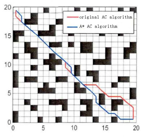
Our algorithm was verified through simulation in three steps. Firstly, the simplified A* search-ACO was compared with the original ACO. Then, the overall performance of dynamic feedback A* search-ACO was contrasted with that of the original ACO. Finally, the path planning effect of our algorithm was investigated under the disturbance of static obstacles.
5.1 Comparison of pheromone initialization
The original ACO was compared with the ACO, in which only the pheromone initialization had been improved. The simulation parameters were initialized as: number of ants in the colony, 30; the maximum number of iterations, 40; $\alpha=1$; $\beta=7$; $\rho=0.12$. Environment 1 was taken as the map, the first raster as the start node, and the 400th raster as the target node. Fifty simulations were conducted and the mean value was obtained. Figure 4 shows the planned paths of these simulations.
Figure 4. The paths planned by the simplified A* search-ACO and the original ACO
Table 2 compares the convergence time, the number of iterations and the optimal path length of the two algorithms.
Table 2. Comparison of the parameters about initial pheromone
|
Algorithm |
Shortest path |
Time |
Number of iterations |
|
Original ACO |
29.32 |
16.26 |
27 |
|
Simplified A* ACO (k=5) |
27.89 |
6.92 |
13 |
|
Simplified A* ACO (k=10) |
27.89 |
3.62 |
6 |
5.2 Overall comparison
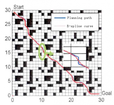
The dynamic feedback A* search-ACO was contrasted with the original ACO using a 30×30 raster map. Raster 1 was taken as the start node and Raster 900 as the end node. The paths planned by the two algorithms are compared in Figure 5 and Table 3.
Figure 5. Smooth path planning of A* ACO (start: start node; goal: target node)
Table 3. Comparison of the path planning results
|
Algorithm |
Shortest path |
Mean path length |
Time |
Mean number of iterations |
|
Original ACO |
49.66 |
51.42 |
56.33 |
42.8 |
|
Simplified A* ACO |
43.91 |
45.82 |
9.72 |
15.1 |
5.3 Path planning under static obstacles
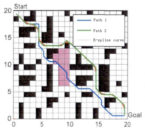
Finally, a simulation was conducted with the following initial conditions: $\alpha=1, \beta=7, \rho=0.12$ and $p_{0}=0.85$. Several obstacles were added after the 10th iteration. Path 1 and path 2 were generated before and after the addition, respectively (Figure 6).
Figure 6. Path planning under static obstacles (start: start node; goal: target node)
As can be seen from Figure 6, A* search-ACO simplified by the initial pheromone achieved fast initial search and output a short optimal path, thus a good search efficiency. Figure 6 also shows that the improved ACO can converge quickly after 10th iterations. The algorithm can adapt to the environment well, because it selects the dynamic control parameter $p_{0}$ according to the feedback on path length. Overall, the simulation results prove that our algorithm can converge to the optimal path quickly, despite the presence of static obstacles.
This paper proposes a smooth path planning method for mobile robots based on closed-loop A* search algorithm and improved ACO, aiming to enhance the search efficiency of the ACO and solve the contradiction between global search ability and convergence speed. The improved ACO outputs a path with a good evaluated cost by simplified A* search algorithm, and increases the initial value of pheromone on the path searched by the A* search algorithm. Finally, the planned path was smoothened by cubic B-spline curve. The simulation results show that the improved ACO found a shorter path within less time than the original ACO.
[1] Wang, M., Liu, J.N.K. (2008). Fuzzy logic-based real-time robot navigation in unknown environment with dead ends. Robotics and Autonomous Systems, 56(7): 25-643. https://doi.org/10.1016/j.robot.2007.10.002
[2] Kamil, Ž., Maxim, V. (2015). Localization and navigation of mobile robot for outdoor area with motion recognition. Robotics & Autonomous Systems, 35(2): 77-96. https://doi.org/10.1016/S0921-8890(00) 00124-X
[3] Mac, T.T., Copot, C., Tran, D.T., Tran, D.T., De Keyser, R. (2017). A hierarchical global path planning approach for mobile robots based on multi-objective particle swarm optimization. Applied Soft Computing, 59: 68-76. https://doi.org/10.1016/j.asoc.2017.05.012
[4] Gao, Y., Xu, H., Hu, M.Q., Liu, J., Liu, J.H. (2017). Path planning under localization uncertainty. Journal Européen des Systèmes Automatisés, 50(4-6): 435-48. https://doi.org/10.3166/JESA.50.435-448
[5] Telesca, L., Lovallo, M. (2012). Analysis of seismic sequences by using the method of visibility graph. Europhysics Letters, 97(5): 50002. https://doi.org/10.1209/0295-5075/97/50002
[6] Ono, M., Pavone, M., Kuwata, Y. (2012). Chance-constrained dynamic programming with application to risk-aware robotic space exploration. Autonomous Robots, 39(4): 555-571. https://doi.org/10.1007/s10514-015-9467-7
[7] Wang, Z.Q., Zhu, X.G., Han, Q.Y. (2011). Mobile robot path planning based on parameter optimization ant colony algorithm. Procedia Engineering, 15(1): 2738-2741. https://doi.org/10.1016/j.proeng.2011.08.515
[8] Lv, T., Feng, M. (2017). A smooth local path planning algorithm based on modified visibility graph. Modern Physics Letters B, 31(19-21): 1740091. https://doi.org/10.1142/S0217984917400917
[9] Sun, G., Bin, S. (2017). Router-level internet topology evolution model based on multi-subnet composited complex network model. Journal of Internet Technology, 18(6): 1275-1283. https://doi.org/10.6138/JIT.2017.18. 6.20140617
[10] Masehian, E., Amin-Naseri, M.R. (2004). A voronoi diagram-visibility graph-potential field compound algorithm for robot path planning. Journal of Field Robotics, 21(6): 275-300. https://doi.org/10.1002/rob.v21:6
[11] Liu, Y.S., Ramani, K., Liu, M. (2011). Computing the inner distances of volumetric models for articulated shape description with a visibility graph. IEEE Transactions on Pattern Analysis & Machine Intelligence, 33(12): 2538-2544. https://doi.org/10.1109/TPAMI.2011.116
[12] Faigl, J., Vonásek, V., Přeučil, L. (2013). Visiting convex regions in a polygonal map. Robotics and Autonomous Systems, 61(10): 1070-1083. https://doi.org/10.1016/j.robot.2012.08.013
[13] Kim, J., Kim, M., Kim, D. (2011). Variants of the quantized visibility graph for efficient path planning. Advanced Robotics, 25(18): 2341-2360. https://doi.org/10.1163/016918611x603855
[14] Tsardoulias, E.G., Iliakopoulou, A., Kargakos, A., Petrou, A. (2016). A review of global path planning methods for occupancy grid maps regardless of obstacle density. Journal of Intelligent and Robotic Systems, 84(1-4): 1-30.
[15] Shao, M.L., Lee, J.Y., Han, C.S., Shin, K.S. (2015). Sensor-based path planning: The two-identical-link hierarchical generalized Voronoi graph. International Journal of Precision Engineering and Manufacturing, 16(8): 1883-1887. https://doi.org/10.1007/s12541-015-0245-4
[16] Yuan, Q., Han, C.S. (2016). Research on robot path planning based on smooth a* algorithm for different grid scale obstacle environment. Journal of Computational and Theoretical Nanoscience, 13(8): 5312-5321. https://doi.org/10.1166/jctn.2016.5419
[17] Akbarimajd, A., Hassanzadeh, A. (2012). Autonomously implemented versatile path planning for mobile robots based on cellular automata and ant colony. International Journal of Computational Intelligence Systems, 5(1): 39-52. https://doi.org/10.1080/18756891.2012.670520
[18] Das, P.K., Behera, H.S., Panigrahi, B.K. (2016). A hybridization of an improved particle swarm optimization and gravitational search algorithm for multi-robot path planning. Swarm & Evolutionary Computation, 28:14-28. https://doi.org/10.1016/j.swevo.2015.10.011
[19] Wang, Y., Cao, W. (2014). A global path planning method for mobile robot based on a three-dimensional-like map. Robotica, 32(4): 14-20. https://doi.org/10.1017/s0263574713000738
[20] Navarro, I., Fernando, M. (2011). A framework for the collective movement of mobile robots based on distributed decisions. Robotics & Autonomous Systems, 59(10): 685-697. https://doi.org/10.1016/j.robot.2011. 05.001
[21] Oleiwi, B.K., Roth, H., Kazem, B.I. (2014). A hybrid approach based on aco and ga for multi objective mobile robot path planning. Applied Mechanics & Materials, 527(527): 203-212. https://doi.org/10.4028/www.scientific.net/amm.527.203
[22] Leach, A.R., Lemon, A.P. (2015). Exploring the conformational space of protein side chains using dead-end elimination and the A* algorithm. Proteins-structure Function & Bioinformatics, 33(2): 227-239. https://doi.org/10.1002/(sici)1097-0134(19981101)33:2<227::aid-prot7>3.0.co;2-f
[23] Sun, G., Bin, S. (2018). A new opinion leaders detecting algorithm in multi-relationship online social networks. Multimedia Tools and Applications, 77(4): 4295-4307. http://dx.doi.org/10.1007/s11042-017-4766-y