Acouri Mourad* | Zennir Youcef | Cherif Tolba
© 2022 IIETA. This article is published by IIETA and is licensed under the CC BY 4.0 license (http://creativecommons.org/licenses/by/4.0/).
OPEN ACCESS
This paper proposes adaptive neuro-fuzzy inference system (ANFIS) to predict the risk with its aggregated cost (CR) of an accident in road transportation of hazardous material, the aim is to provide a more accurate and reliable data for the safety of transportation. The determination risk index by the conventional methods such as Risk graphs and deterministic approaches may lead to imprecise values due to the uncertainties, in both parameters and models. The proposed technique is a hybrid schema, which combines the main advantageous of fuzzy logic (address uncertainties) and neural network (learn from a given data). In other hand our study seeks to tune the parameters of the proposed model by particle swarm optimization (PSO), firefly algorithm (FA), imperialist competitive algorithm (ICA) and human based-behavior optimization (HBBO) and hence optimize the performance of ANFIS. The simulation result of this work and the comparative analysis shows that ANFIS yield height performance and the ANFIS-PSO was the outstanding one in the training phase, while ANFIS-FA gives better results in the testing process.
CR, hazmat, PSO, FA, HBBO, ICA
With the progress of industrial societies the requirement of logistics industry, notably the hazardous material, which differ from the simple one and may entails a potential risk for the safety of both human and environment, has increased progressively [1, 2]. In order to meet those requirement the government agencies has attempt to make some specific countermeasures by enhancing the safety of expressways and extending the road network, however several challenges (network design studies, risk modeling studies, development of decision support systems, facility location studies, integrated location and routing studies, and vehicle routing and scheduling studies...) should be carefully treated, where the accurate data are primordial.
Over the last few years there has been growing concern regarding the risk of accident in road transportation of hazmat, especially due to the road congestion and its effect became more and more complicated. the risk of road accident in the transportation of hazmat may give rise to other risks (risk of fire, explosion and material leakage) depending on the type of the transported material and may causes a serious damage on both humans, environment and economic.
In effect, one of the most prominent tool that can used in transportation process is vehicle routing problem. Vehicle routing is a selection of shortest path generally solved as bi-objective problems, usually by integer programming and by heuristic approaches [3]. Those studies are based on rather deterministic approaches and several criteria (probability of accidents, the population affected by accidents, the population distribution (on-road and off- road population), population fluctuation, traffic flows etc.) should be considered with accurate and precise data, which is difficult to posse it. It is worthy to mention that fuzzy logic (FL) adequately address uncertainties and ambiguities and adopted in many studies. Zhao and Cao [2] proposed Fuzzy Random Chance Constrained Programming Model for the Vehicle Routing Problem of Hazardous Materials Transportation. Men et al. [4] investigate a chance constrained programming approach for hazmat capacitated vehicle routing problem in Type-2 fuzzy environment.
Indeed other drawback comes to exacerbate the determining of risk and its cost (the main objective considered in vehicle routing problem) in hazmat transportation, which is each criteria that influence the definition of risk and its cost varies from road to road and from season to season. Here it should be kept in mind that no states, regions or cities are capable to provide such thing, and therefore the amount and quality of data required differ from region (network) to region (network) and usually they are time dependent (seasons, days …) [3]. Neural network might be an ideal alternative to handle with those changes because of its ability to adapt its weight from a given real data.
Indeed, other effective tool that can used in transportation process is risk assessment. Risk assessment is a study of probability of risk occurrence and its consequences, many of study have been conducted in this field [5, 6]. Chen et al. [7]. Have introduced Bayesian network (BN) to predict the accident of handling time to enhance the performance of emergency rescue in transportation accidents of hazardous materials. Weng et al. [8] developed a quantitative risk assessment for the hazmat transportation accident in which the possible accident scenarios are identified by an event tree with help of six intermediate events. Ghaleh et al. [9]. In their research job hazard analysis (JHA) method was proposed to identify the safety risk contributing factors (SRCFS) and sub-safety risk contributing factors (Sub-SRCFS) of road oil trucks, then fuzzy analytical hierarchy process (FAHP) was used to rank the identified SRCFS and Sub-SRCFS and finally the safety risk assessment pattern in road oil truck was conducted by performing failure modes and effect analysis (FMEA) approach [10]. Have conducted a Quantitative Assessment for the Safety and Health Risks in HAZMAT Road Transport, in their study a Bayesian network and the fuzzy inference system have been used to evaluate the severity of health and safety consequences of material leakage from trucks [11]. Have analyzed the factors that influences hazardous material transportation accidents based on Bayesian networks [12]. Analyzed the risk factors for high-speed railway station in China using fault tree method (FTA) then transform it into fuzzy petri net (FPN), additionally Risk control model with the minimum safety risk level and minimum necessary cost as the objectives was also built up and solved by discrete particle swarms optimization algorithm. Nevertheless the most proposed methods have been made after several assumption and do not reflect reality.
Motivated by this fact our study aims to predict the CR value by adopting the standard of ANFIS model. All the parameters of the proposed approach was optimized by PSO, FA, ICA and HBBO. The applied model was tested and validated based on the data set of road network in Belgrade city Serbia. The Root Mean Square Error (RMSE) and mean square error (MSE) are considered to test the degree of accuracy of the proposed model. The obtained results of numerical simulation prove the efficiently of the ANFIS model to predict the CR and the comparison results shows that ANFIS-PSO gives height training ability (training phase), while ANFIS-FA yields better performance in testing case.
The rest of the paper is organized as follows. The main steps of proposed model to predict the CR value and its optimization phase are explained in Section 2. Section 3 provide the mathematical background of ANFIS model, which highlight how to map from the parameters entries (Inputs) to the output (CR) via 5 layers. In Section 4 and its subsections gives a brief description of the proposed algorithms to optimize the performers of ANFIS. Finally, in Sections 5 and 6 results and conclusions are explained respectively.
The risk of accident in road transportation of hazardous material can occur due to various mechanisms, and it is significantly dependent on human factors, environmental conditions, management factors and the equipment Failure. Different accident scenarios may result from a combination of events following road accident depending on the type of transported substance (explosion, fire and the release of toxic material). The damage resulting from road accidents gives rise to a number of consequences, which are classified in three main categories (environment, social and economic) see Figure 3.
In order to estimate the risk of accident aggregate with its cost this paper proposes a method based on ANFIS model, which is based on three main steps see Figure 1.
In the first phase the criteria (inputs) that influences the value of the CR are identified. The inputs and their descriptions are illustrated in Table 1. After that the road network on which the value of the input parameters and the output (CR) are given on each branch that separate the node (client, depot station ...) must be selected.
Figure 1. Main steps of ANFIS for determinng the CR value
Figure 2. ANFIS based PSO, FA, ICA and HBBO
Table 1. Criteria for defining the CR values on a transport network of city roads [3]
|
Inputs |
Description of inputs |
|
The carrier’s operating costs (X 1 ∈ [0,7500]) |
The cost of operator carrier is mainly computed according to the value of time, distance, cost of fuel etc. In this study carrier, operating costs is given based on the length of the road [13]. |
|
Fire Fighters response (X 2 ∈ [0,15]) |
Fire fighters response depend entirely on Traveled distance (Lij) and the costs of the transportation c (fuel consummation for example), which is given by: Lij* c. Fire fighters response is the necessary time taken by of emergency services to arrive at the location of accident. The average reaction time is expressed in this study in minutes, which is relative to the distance that separate emergency services center to the hot spot. |
|
Losses related to the environment (X 3 ∈ [0,5]) |
This is the number of environment's critical point (Headwaters Rivers, Agricultural Urban, Forest fragment) that can be affected by the accident. These stragicals points that are within 800m from the accident location are taken into account [14]. |
|
Risk of an accident (X 4 ∈ [0,1]) |
Risk of an Accident is determined according to of the number of accident (f 1) recorded in database of the concerned road over the last 10 years. the number of branches (f 2), the percentage of heavy cars in the traffic (f 3) and the level of signaling (f 4). The total Risk of an Accident (X 4) is computed based on this equation X4 = 0.3 f1/ f1max + 0.2 f2/ f2max + 0.2 f3/ f3max + 0.3 f4/ f4max. the value of f4 is given by this following scale: 1 – traffic rules, 2 – regulation by means of traffic signs, 3 – regulation by means of light signals. |
|
The gravity related to an accident (X 5 ∈ [0,9500]) |
Is given according the affected population who lives around the accident's zone. The control zone is determined as mentioned in the factor X3. |
|
Losses related to the stratigical points (X 6 ∈ [0,10]) |
Risk related with stragicals point is the number of important infrastructures presented in the accident’s locations (railways, electric lines, industrial, commercial and transport facilities, schools, hospitals). |
|
Risk of terror attack/hijack (X 7 ∈ [1,5]) |
Risks of terror attack is the consequences that caused by an eventual attack of terrorist in the control zone and its value is determent by adopting this following scale: 1- very low, 2 – low, 3 – moderate, 4 – height 5 – very height. |
Figure 3. Hierarichal framwork of causes and consequances of raod accident
In the second step the type of the ANFIS and the membership function of each input and output must be selected then the first model is generated in order to map from the inputs to the output by the means of fuzification, product, normalization and defuzification layers (section 2 highlight how to map from the input parameters to the CR).
In order to optimize the performance of the proposed method and avoid the inclusion of expert for the designing parameters of the ANFIS four algorithm from meta-heuristic optimization (PSO, FA, ICA and HBBO) are used to tune the main parameters of ANFIS (the mean and variance of Gaussian membership function and the constant pi, qi and ri. See Figure 2). Finally after the termination criteria of the tuning process (the number of iterations) are satisfied then ANFIS model is ready to be used.
The ANFIS is a hybrid algorithm proposed by Jang [15], it combine the fuzzy logic with neural network. This integration allows to the model to combine the main advantages of FL (approximate reasoning) and neural network (Learning from examples) and overcome their disadvantages, which are no adaptability (soliciting the opinion of experts) and difficulties of describing knowledge. Figure 4 shows a typical ANFIS structure which consists of five distinct layers.
Figure 4. The ANFIS architecture for estimating the CR of hazmat road transportation
Considering first-order Takagi–Sugeno fuzzy type with two inputs x and y and one output f then its fuzzy rules can be expressed by:
if $\mathrm{x}$ is $\mathrm{A}_{\mathrm{i}}$ and $\mathrm{y}$ is $\mathrm{B}_{\mathrm{i}}$ then $\mathrm{f}_{\mathrm{i}}=\mathrm{p}_{\mathrm{i}} \mathrm{x}+\mathrm{q}_{\mathrm{i}} \mathrm{y}+\mathrm{r}_{\mathrm{i}}$ (1)
where, $\mathrm{A}_{\mathrm{i}}$ and $\mathrm{B}_{\mathrm{i}}$ indicate the fuzzy sets, and $\mathrm{p}_{\mathrm{i}}$, $\mathrm{q}_{\mathrm{i}}$ and $\mathrm{r}_{\mathrm{i}}$ respectively represent the parameters that will be obtained by a given algorithm in the training phase. The output of the ANFIS model is the weighted average of outputs of all nodes. The $\mathrm{O}_{\mathrm{i}}^{\mathrm{j}}$ denotes the output of ith node in layer j [16].
The first layer represents the inputs of ANFIS model, which are Fuzzified with the means of fuzzy variable for each input. The output of each node of this layer is the membership value.
$\mathrm{O}_{\mathrm{i}}^1=\mu_{\mathrm{A}_{\mathrm{i}}}(\mathrm{x})$ (2)
$\mathrm{O}_{\mathrm{i}}^1=\mu_{\mathrm{B}_{\mathrm{i}}}(\mathrm{y})$ (3)
where, $\mu_{\mathrm{A}_{\mathrm{i}}}(\mathrm{x})$ and $\mu_{\mathrm{B}_{\mathrm{i}}}(\mathrm{y})$ indicates its respective fuzzy membership function. x and y are the input of node and $\mathrm{A}_{\mathrm{i}}$ and $\mathrm{B}_{\mathrm{i}}$. Gaussian MFs were used in this study to describe the inputs variables.
$\mu_{\mathrm{A}_{\mathrm{i}}}=\exp \left(-\frac{1}{2}\left(\frac{\mathrm{x}-\mathrm{c}_{\mathrm{i}}}{\sigma_{\mathrm{i}}}\right)^2\right)$ (4)
where, $\mathrm{c}_{\mathrm{i}}$ and $\sigma_i$ represents respectively the mean and the variance of the membership function, respectively. Typically, the output of this layer is the degree of membership function.
Second layer is the product layer, which multiplies the output of the previous layer with the help of AND operator:
$\mathrm{O}_{\mathrm{i}}^2=\mathrm{w}_{\mathrm{i}}=\mu_{\mathrm{A}_{\mathrm{i}}}(\mathrm{x})^* \mu_{\mathrm{B}_{\mathrm{i}}}(\mathrm{y})$ (5)
where, $\mathrm{w}_{\mathrm{i}}$ represents the normalized firing strength.
Third layer is normalization layer: a normalization operation is carried out to give:
$\mathrm{O}_{\mathrm{i}}^3=\overline{\mathrm{w}}_{\mathrm{i}}=\frac{\mathrm{w}_{\mathrm{i}}}{\sum \mathrm{w}_{\mathrm{i}}}$ (6)
where, $\overline{\mathrm{w}}_{\mathrm{i}}$ represents the normalized firing strength.
Forth layer represent defuzzification layer: all incoming signals to each input of this layer are difuzzificated via this function:
$\mathrm{O}_{\mathrm{i}}^4=\overrightarrow{\mathrm{w}}_{\mathrm{i}} * \mathrm{f}_{\mathrm{i}}=\overline{\mathrm{w}}_{\mathrm{i}} * \left(\mathrm{p}_{\mathrm{i}} \mathrm{x}+\mathrm{q}_{\mathrm{i}} * \mathrm{y}+\mathrm{r}_{\mathrm{i}}\right)$ (7)
Finally, the fifth layer is the output layer: All signals of this layer are aggregated according to this following function:
$\mathrm{O}_{\mathrm{i}}^5=\sum_{\mathrm{i}}^{\mathrm{n}} \overline{\mathrm{w}}_{\mathrm{i}} * \mathrm{f}_{\mathrm{i}}=\frac{\sum_{\mathrm{i}} \mathrm{w}_{\mathrm{i}} * \mathrm{f}_{\mathrm{i}}}{\sum_{\mathrm{i}} \mathrm{w}_{\mathrm{i}}}$ (8)
4.1 Particle swarm optimization (PSO)
PSO is nature-inspired methods, which is included in swarm-based techniques. It is based on a simple mathematical model, introduced by Kennedy and Eberhart in 1995 [17]. PSO imitate the social behavior of swarm when fling and seeking to reach a destination. It employs a number of particles (candidate solutions) which explore a given search space to find the best solution (i.e. the global best solution). Meanwhile, they update the best location (personal best solution) of each candidate in their paths. In other words, each particle moves through the decision space based on the individual and global best positions. In this algorithm the position (ANFIS parameters) of each particle are updated based on Eq. (9)-(10).
$\mathrm{V}_{\mathrm{i},}^{\mathrm{t}+1}=\mathrm{w} \mathrm{V}_{\mathrm{i}}^{\mathrm{t}}+\mathrm{c}_1 \mathrm{r}_{1 \mathrm{i}}^{\mathrm{t}}\left(\mathrm{p}_{\mathrm{i}, \text { best }}^{\mathrm{t}}-\mathrm{x}_{\mathrm{i}}^{\mathrm{t}}\right)+\mathrm{c}_2 \mathrm{r}_{2 \mathrm{i}}^{\mathrm{t}}\left(\mathrm{G}_{\text {best }}^{\mathrm{t}}-\mathrm{x}_{\mathrm{i}}^{\mathrm{t}}\right)$ (9)
$\mathrm{X}_{\mathrm{i},}^{\mathrm{t+1}}=\mathrm{V}_{\mathrm{i},}^{\mathrm{t}+1}+\mathrm{x}_{\mathrm{i}, \mathrm{j}}^{\mathrm{t}}$ (10)
where: $\mathrm{V}_{\mathrm{i},}^{\mathrm{t}+1}$, $\mathrm{V}_{\mathrm{i}}^{\mathrm{t}}$, indicate the velocity of each particles at the current iteration and previous iteration, $\mathrm{X}_{\mathrm{i}}^{\mathrm{t}+1}$ and $\mathrm{x}_{\mathrm{i}}^{\mathrm{t}}$ denotes the position of particles in current and previous iteration respectively, $\mathrm{p}_{\mathrm{i}, \mathrm{best}}^{\mathrm{t}}$ and $\mathrm{G}_{\text {best }}^{\mathrm{t}}$ represents the personal and the global best of each candidate and the hole swarm, w, $\mathrm{c}_{1,2}$ and r1,2 are respectively the Inertia Weight, personal and global learning coefficient and random number.
4.2 Firefly algorithm (FA)
FA is bio-inspired meta-heuristic algorithm, which belong to swarm optimization technique. It was firstly developed by Yang in late 2007 and 2008 [18]. This algorithm is inspired by flashing pattern and behavior of fireflies at night. It engages a number of fireflies (candidate solutions) which fly around in the search space and move toward the attractive one based on its brightness regardless of their sexes, which constitute the best solution (i.e. the optimal position). It is worthy to notice that the dynamics of fireflies can be reduced to the dynamics of Particle swarm optimization, Harmony Search, simulating Annealing and differential evolution, which gains the ability of the automatic subdivision. The position of fireflies is computed according to the Eq. (11).
$\mathrm{x}(\mathrm{t}+1)_{\mathrm{i}}^{\mathrm{k}}=\mathrm{x}(\mathrm{t})_{\mathrm{i}}^{\mathrm{k}}+\beta_0 \exp \left(-\gamma \mathrm{r}_{\mathrm{ij}}^2\right)\left(\mathrm{x}(\mathrm{t})_{\mathrm{j}}^{\mathrm{k}}-\mathrm{x}(\mathrm{t})_{\mathrm{i}}^{\mathrm{k}}\right)+\alpha\left(\mathrm{r}-\frac{1}{2}\right)$ (11)
with
$\beta(\mathrm{r})=\beta_0 \exp \left(-\gamma \mathrm{r}_{\mathrm{ij}}^{\mathrm{m}}\right) ; \mathrm{m}<1$ (12)
$r_{i j}=\left\|x_j-x_i\right\|=\sqrt{\sum_{k=1}^d\left(x_j^k-x_i^k\right)^2}$ (13)
where: $\beta(\mathrm{r})$ indicates the attractiveness of firefly, $\beta_0$ represents the attractiveness of firefly at $\mathrm{r}=0$, Coefficient of light absorption, $\mathrm{x}_{\mathrm{i}}^{\mathrm{k}}$ is the position of ith firefly at the kth dimension, $\mathbf{x}_{\mathrm{j}}^{\mathrm{k}}$ denotes the position of the jth firefly at the kth dimension, $\mathrm{r}_{\mathrm{ij}}$ is the distance between $\mathrm{x}_{\mathrm{i}}$ and $\mathrm{x}_{\mathrm{j}}$, t iteration, r random number, α randomization parameter.
4.3 Human based behavior optimization (HBBO)
HBBO is a new meta-heuristic optimization proposed by Ahmadi in the late of 2016 [19]. It imitates the behavior of humans in getting success in their life. Humans looks for the success in several fields (music, paint, engineering…), and after the domain of interest is opted based on their purposes and passion they moves to the expert to improve and excel their ability and hence gains more success.
HBBO in its first phase initialize set of population (candidate) and randomly spread them in deferent fields and the number of initial people in each field is obtained by:
N.Ind ${ }_i=$ round $\left\{\frac{N_{\text {pop }}}{N_{\text {field }}}\right\}$ (14)
where, $\mathrm{N}_{\text {pop }}$ and $\mathrm{N}_{\text {field }}$ are respectively the number candidates and fields.
In the second phase (education phase) this algorithm describe how the population move toward expert in their deferent fields. The experts are the candidates who possess the best solution. Each candidate will converge toward its relevant expert based on the spherical coordinate system which is given by:
$\mathrm{x}_{\mathrm{ind}}^{\mathrm{t}+1}=\mathrm{x}_{\mathrm{ind}}^{\mathrm{t}}+\mathrm{r} \cdot\left(\mathrm{k}_2-\mathrm{k}_1\right) \cdot\left(\mathrm{x}_{\mathrm{exp}}^{\mathrm{t}}-\mathrm{x}_{\mathrm{ind}}^{\mathrm{t}}\right)$ (15)
With $\mathbf{x}_{\text {ind }}^{\mathrm{t}+1}$ and $\mathrm{x}_{\mathrm{ind}}^{\mathrm{t}}$ denotes respectively the current and previous position of individuals, $\mathrm{x}_{\mathrm{exp}}^{\mathrm{t}}$ represent the position their expert, r is random variable, $\mathrm{k}_1$ and $\mathrm{k}_2$ are a constant.
After that in the consultation phase individuals may find within society an advisor who can change their minds and therefore they may changes their field. This consultation can be effective if we get a furthermore best solution consequently advisors changes the candidate of solution, otherwise nothing will be changed. The number of decision variable (parameters of ANFIS) that will be changed during this phase is computed in Eq. (16).
$\mathrm{N}_{\mathrm{c}}=\operatorname{round}\left(\sigma . \mathrm{N}_{\mathrm{var}}\right)$ (16)
where, $\mathrm{N}_{\mathrm{var}}$ is the total number of decision variable and $\sigma$ is a constant.
In the fourth phase (field changing probability) HBBO firstly ranks and sort the expert individuals based on their fitness score then calculate the changing probability by:
$\mathrm{p}_{\mathrm{i}}=\frac{\mathrm{O}_{\mathrm{i}}}{\mathrm{N}_{\text {field }}+1}$ (17)
where, $\mathrm{p}_{\mathrm{i}}$ and $\mathrm{O}_{\mathrm{i}}$ are ranking probability and the index of the ith sorted field, respectively. After that a random variable (rand) between 0 and 1 is generated, this comparison is performed:
if rand $\leq \mathrm{p}_{\mathrm{i}} \rightarrow$ field changing occurs (18)
In this phase, a selection probability for every person is computed by:
$\mathrm{P}_{.} \mathrm{S}_{\mathrm{j}}=\left|\frac{\mathrm{f}\left(\text { individual }_{\mathrm{j}}\right)}{\sum_{\mathrm{k}=1}^{\text {Nind }} \mathrm{f}\left(\text { individual }_{\mathrm{k}}\right)}\right|$ (19)
With $\mathrm{f}\left(\right.$individual$_{\mathrm{j}}$) is the fitness score of the jth people and Nind is the number of people in the selected field. Finally, by adopting the roulette wheel selection technique [20], a candidate will be selected and moves to a random field.
Finally, like others algorithms HBBO perform the Finalization step (check the termination criteria).
4.4 Imperialist competitive algorithm (ICA)
ICA is a novel evolutionary algorithm originally developed by Atashpaz-Gargari and Lucas [21]. It mimics the imperialistic competition. The essence of this algorithm can be attained in 5 main steps (empire initialization, assimilation, revolution, imperialist competition and finalization).
In the first phase like other algorithms ICA generate randomly an initial population (countries), the countries with best score are called imperialists and the others are known as colonies, then spread them among other imperialist based on their relevant power, and by performing roulette wheel selection [20, 22] an initial empire will be formed. The number of imperialists is obtained by:
$\mathrm{N}_{\text {imp }}=\operatorname{round}\left\{\frac{\mathrm{N}_{\text {pop }}}{\mathrm{N}_{\mathrm{emp}}}\right\}$ (20)
With $\mathrm{N}_{\text {pop}}$ and $\mathrm{N}_{\mathrm{emp}}$ indicate the number of population and empires.
After that in the second phase (assimilation phase) all colonies moves to reach the position of their imperialist based on uniform distribution written in Eq. (21).
$\mathrm{x} \sim \mathrm{U}\left(\mathrm{x}_{\mathrm{col}}^{\mathrm{t}}, \beta \times \mathrm{d}\right)$ (21)
where, $\mathrm{x}_{\mathrm{col}}^{\mathrm{t}}$, $\beta$ and $\mathrm{d}$ denotes respectively the current position of colony, is assimilation coefficient and d is the distance between colony and its imperialist.
In the revolution phase (third phase) each country among empires seeks to increase their power by changing the position of their decision variable. During this phase the number of variable that will be changed are determined according to Eq. (16). Then the selected variables of imperialists are updated based on normal distribution described in Eq. (23), while for colonies a predefined probability (pc) is firstly considered after that a random variable (r) between 0 and 1 is generated then a comparison depicted in Eq. (22) is performed and if this comparison is verified they update their position based on Eq. (23).
if $\mathrm{r} \leq \mathrm{pc} \rightarrow$ rovolution process occurs (22)
$\theta \sim \mathrm{N}\left(\mathrm{x}_{\mathrm{imp}, \mathrm{col} \quad}^{\mathrm{t}}, \gamma \cdot\left(\mathrm{x}_{\max }-\mathrm{x}_{\min }\right)\right)$ (23)
where, $\theta$ indicate a new position, $\mathbf{x}_{\mathrm{imp}, \mathrm{col}}^{\mathrm{t}}$ is the current position of imperialist and colony, $\gamma$ is revolution rate, $\mathrm{x}_{\max }$ and $\mathbf{x}_{\min }$ denotes the upper and lower bond of the decisions variable. Here it is worthy to notice that during this phase a colony may reach better position than its imperialist therefore it became a new leader of its relevant empire.
In order to perform the fourth step the total power of each empire is determined at each iteration by Eq. (24).
$\mathrm{TC}_{\mathrm{n}}=\operatorname{cost}\left(\right.$imperialist$\left._{\mathrm{n}}\right)+\xi \operatorname{mean}\left\{\operatorname{cost}\left(\right.\right.$colonies$\left.\left._{\mathrm{n}}\right)\right\}$ (24)
where, $\mathrm{TC}_n$ denote the total cost of an nth empire and ξ represent a positive number which is considered to be less than 1.
In the fourth phase (empire competition) each empire seeks to takes possession of the weakest colonies of other empire. The more colonies in empire the strongest it becomes the fewer colonies in empire the weaker it becomes. In this phase a weakest colony is firstly selected then the probability selection is calculated by:
$\mathrm{p}_{\mathrm{jemp}}=\exp \left(-\alpha \frac{\mathrm{TC}_{\mathrm{jemp}}}{\sum_{\mathrm{k}=1}^{\mathrm{Nemp}} \quad \mathrm{TC}_{\mathrm{k}}}\right)$ (25)
With $\mathrm{p}_{\text {jemp }}$ is the probability selection of the jth empire, $\alpha$ is the selection pressure and $\mathrm{TC}_{\text {jemp }}$ is a total power of jth empire. Finally based on the roulette wheel selection the winner empire is determined hence it possess the selected colony. The empires that are not able to gain more colonies collapses and therefore became a colony of other empires.
In the last phase of these algorithm (finalization) the above-mentioned process from phase 2 are repeated until the termination criteria are verified.
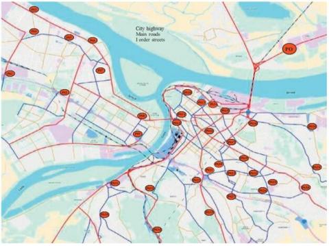
In order to validate and test the performance of the ANFIS model we used the data provided from a study of the distribution of oil and oil derivatives in Belgrade, Serbia. this study was conducted on the road network with a total length of 863 Km and only the potential road with a width of 5Km minimum are taken into consideration. In this road network the oil and its derivative was transported from a Pancevo Oil Refinery (POI) to a 36 fuel station (NIS) (see Figure 5). in this study the data of the parameters (inputs and output) of each branch that links the NIS stations to the POI are obtained on the basis of data on the environmental quality of the city of Belgrade in 2013 and the General Urban Plan of Belgrade for the period until 2021 (see Table 2) [3].
In the present study, a classical fuzzy model on the basis of the fuzzy c-means clustering algorithm was selected. All subsequent processing and modeling were carried out using Matlab software and associated tools. Accordingly, 7 characteristics (the carrier operating cost, emergency response, losses associated with environment, risk of an accident, the consequence of an accident, losses associated with infrastructure and risk of terror attack) were used to estimate CR value. 0.7 of data sets were randomly selected for training stages, and another subset consisted of 0.3 of data sets left for validation step. Takagi–Sugeno fuzzy structure was used based on fuzzy c-means clustering method with 15 clusters for CR value. 250 candidate and 1000 iterations were used to test the proposed algorithms.
The PSO’s parameter are Inertia w=0.7, c1=1, c2=2.
The FA’s parameter are Light γ=1, $\beta_0$=2, α=0.2*0.98.
The HBBO’s parameter are Nfields=50, K1=0, K2=2.5, σ=0.2.
The ICA’s parameter are Nemp=50, α=1, β=1.5, pc=0.05, γ=0.1, ξ=0.2.
The description of the inputs that considered are reported in Table 1.
Basically, when a new hybrid model is proposed, its performance should be tested for both training and testing phases. The training process indicate the capability of the model to fit the data, while the testing/validation shows the power of estimation of the proposed model [22, 23].
Figure 5. The raods that links the POI to NIS stations [3]
Table 2. The values of the inputs (criteria) and CR of the segments that links POI to NIS [1]
|
X1 |
X2 |
X3 |
X4 |
X5 |
X6 |
X7 |
CR |
X1 |
X2 |
X3 |
X4 |
X5 |
X6 |
X7 |
CR |
|
650.9 |
5.88 |
4 |
0.48 |
5387 |
5 |
1 |
6.60 |
857.6 |
9.46 |
4 |
0.58 |
4222 |
5 |
5 |
6.85 |
|
968.3 |
6.97 |
2 |
0.26 |
5315 |
9 |
3 |
6.42 |
245.1 |
3.78 |
4 |
0.67 |
4935 |
9 |
1 |
7.01 |
|
712.7 |
5.17 |
2 |
0.70 |
5175 |
5 |
3 |
6.76 |
394.7 |
8.73 |
3 |
0.65 |
8086 |
1 |
1 |
7.16 |
|
1478.4 |
12.49 |
2 |
0.56 |
8508 |
6 |
5 |
6.96 |
456.8 |
11.73 |
5 |
0.23 |
6644 |
1 |
1 |
7.00 |
|
895.3 |
7.26 |
4 |
0.45 |
5079 |
1 |
3 |
6.75 |
1127.5 |
7.27 |
1 |
0.58 |
4302 |
9 |
1 |
6.19 |
|
581.1 |
5.71 |
2 |
0.44 |
4587 |
6 |
2 |
5.81 |
509.2 |
9.58 |
2 |
0.37 |
5910 |
9 |
5 |
6.95 |
|
905.9 |
12.12 |
1 |
0.64 |
6527 |
4 |
2 |
6.95 |
247.9 |
11.98 |
3 |
0.66 |
5864 |
3 |
1 |
7.11 |
|
383.7 |
10.59 |
4 |
0.78 |
4766 |
10 |
1 |
6.82 |
302.4 |
6.65 |
5 |
0.28 |
6735 |
2 |
5 |
6.82 |
|
114.2 |
2.82 |
2 |
0.55 |
7300 |
10 |
2 |
6.77 |
413.7 |
6.83 |
3 |
0.67 |
7548 |
1 |
3 |
7.01 |
|
107.7 |
11.90 |
4 |
0.89 |
6544 |
6 |
1 |
6.91 |
447.8 |
11.42 |
3 |
0.83 |
4234 |
3 |
1 |
7.15 |
|
119.5 |
5.10 |
4 |
0.89 |
6766 |
5 |
3 |
6.87 |
399.1 |
11.84 |
5 |
0.86 |
7002 |
9 |
4 |
8.21 |
|
509.1 |
4.59 |
3 |
0.85 |
8250 |
1 |
3 |
7.11 |
129.6 |
6.53 |
1 |
0.61 |
9488 |
7 |
5 |
7.05 |
|
495.7 |
8.73 |
4 |
0.81 |
7065 |
6 |
5 |
7.18 |
261.8 |
12.93 |
4 |
0.81 |
6606 |
3 |
4 |
7.26 |
|
419.2 |
7.93 |
2 |
0.70 |
4027 |
6 |
5 |
7.05 |
365.2 |
10.21 |
2 |
0.30 |
8281 |
2 |
4 |
6.83 |
|
53.7 |
6.22 |
4 |
0.91 |
7893 |
6 |
5 |
6.87 |
192.4 |
4.14 |
5 |
0.34 |
6866 |
10 |
4 |
6.99 |
|
488.9 |
12.45 |
5 |
0.45 |
7654 |
10 |
1 |
6.70 |
317.6 |
2.66 |
2 |
0.62 |
5452 |
10 |
5 |
7.07 |
|
689.5 |
8.39 |
5 |
0.85 |
7969 |
3 |
5 |
7.24 |
185.4 |
4.29 |
5 |
0.67 |
4182 |
6 |
2 |
7.00 |
|
479.2 |
10.73 |
3 |
0.64 |
9213 |
5 |
1 |
6.95 |
337.1 |
4.38 |
4 |
0.28 |
6227 |
1 |
4 |
6.32 |
|
1267.9 |
10.16 |
5 |
0.75 |
4683 |
10 |
3 |
7.11 |
503.6 |
4.06 |
3 |
0.44 |
8518 |
2 |
4 |
6.77 |
|
1003.7 |
5.07 |
3 |
0.70 |
4497 |
10 |
1 |
7.00 |
323.5 |
3.53 |
2 |
0.74 |
4859 |
6 |
2 |
6.28 |
|
361.8 |
12.08 |
5 |
0.24 |
6670 |
1 |
5 |
6.81 |
476.3 |
8.92 |
5 |
0.93 |
7989 |
9 |
3 |
7.53 |
|
501.2 |
4.74 |
5 |
0.27 |
9076 |
8 |
4 |
6.93 |
226.4 |
2.98 |
3 |
0.80 |
6314 |
1 |
5 |
7.07 |
|
3056.7 |
12.20 |
4 |
0.36 |
6469 |
10 |
3 |
7.20 |
401.8 |
10.09 |
2 |
0.58 |
4831 |
7 |
5 |
7.00 |
|
562.7 |
4.90 |
1 |
0.84 |
4084 |
2 |
5 |
6.70 |
254.3 |
12.70 |
5 |
0.21 |
5315 |
1 |
4 |
6.94 |
|
211.5 |
7.94 |
2 |
0.92 |
7530 |
1 |
3 |
7.16 |
317.8 |
5.14 |
2 |
0.51 |
5822 |
7 |
1 |
5.97 |
|
743.7 |
10.43 |
2 |
0.78 |
4129 |
5 |
2 |
6.99 |
371.5 |
5.72 |
3 |
0.77 |
8006 |
3 |
5 |
6.79 |
|
1248.4 |
10.12 |
1 |
0.69 |
7781 |
8 |
2 |
7.02 |
751.3 |
11.64 |
2 |
0.46 |
8637 |
8 |
4 |
6.95 |
|
1089.7 |
6.31 |
2 |
0.55 |
5425 |
5 |
2 |
6.31 |
1112.6 |
12.30 |
5 |
0.53 |
5420 |
3 |
4 |
7.01 |
|
117.1 |
7.19 |
3 |
0.75 |
7129 |
10 |
2 |
6.95 |
461.3 |
8.10 |
1 |
0.72 |
6281 |
5 |
1 |
6.39 |
|
202.2 |
2.83 |
0 |
0.94 |
6860 |
7 |
4 |
6.90 |
503.4 |
5.32 |
2 |
0.50 |
8371 |
9 |
4 |
6.93 |
|
363.9 |
11.62 |
5 |
0.54 |
8469 |
7 |
1 |
6.79 |
119.8 |
7.83 |
3 |
0.28 |
5998 |
5 |
5 |
6.81 |
|
1089.5 |
11.57 |
3 |
0.76 |
4845 |
2 |
5 |
7.07 |
95.7 |
2.64 |
4 |
0.28 |
3950 |
6 |
3 |
6.12 |
|
495.8 |
12.20 |
1 |
0.52 |
8393 |
4 |
3 |
7.14 |
96.2 |
7.06 |
1 |
0.64 |
7929 |
2 |
1 |
6.22 |
|
491.2 |
7.66 |
5 |
0.69 |
8659 |
6 |
3 |
6.88 |
271.6 |
6.22 |
3 |
0.32 |
8648 |
3 |
5 |
6.91 |
|
1156.7 |
9.23 |
4 |
0.65 |
9279 |
7 |
4 |
7.46 |
531.6 |
10.83 |
1 |
0.29 |
4842 |
4 |
1 |
5.17 |
|
1257.2 |
6.87 |
1 |
0.42 |
8445 |
7 |
1 |
6.05 |
413.1 |
11.23 |
1 |
0.57 |
6540 |
7 |
4 |
7.05 |
|
302.6 |
5.68 |
2 |
0.26 |
6979 |
4 |
2 |
5.35 |
103.5 |
11.43 |
4 |
0.74 |
5956 |
7 |
5 |
7.35 |
|
393.5 |
6.59 |
3 |
0.92 |
4025 |
1 |
3 |
7.04 |
1008.2 |
8.15 |
2 |
0.94 |
7725 |
9 |
2 |
6.91 |
|
627.1 |
5.82 |
3 |
0.22 |
6471 |
9 |
5 |
7.06 |
2157.9 |
3.91 |
4 |
0.72 |
8622 |
4 |
1 |
6.90 |
|
798.5 |
8.22 |
3 |
0.85 |
6240 |
10 |
5 |
7.06 |
627.1 |
3.03 |
2 |
0.63 |
4829 |
3 |
3 |
6.01 |
|
1003.8 |
6.34 |
4 |
0.77 |
8640 |
8 |
4 |
7.20 |
210.9 |
7.25 |
5 |
0.23 |
5541 |
1 |
1 |
6.03 |
|
508.4 |
12.31 |
1 |
0.43 |
7816 |
7 |
2 |
6.82 |
216.3 |
6.50 |
2 |
0.38 |
7508 |
10 |
2 |
6.82 |
|
498.2 |
11.68 |
2 |
0.57 |
7116 |
8 |
3 |
7.04 |
511.4 |
6.49 |
5 |
0.84 |
7276 |
7 |
5 |
7.16 |
|
95.7 |
10.71 |
1 |
0.89 |
6453 |
10 |
3 |
7.11 |
458.1 |
10.09 |
2 |
0.94 |
4825 |
2 |
3 |
7.12 |
|
406.8 |
6.40 |
1 |
0.86 |
7191 |
10 |
5 |
6.64 |
592.8 |
8.42 |
3 |
0.84 |
4018 |
9 |
4 |
6.93 |
|
571.5 |
9.18 |
4 |
0.91 |
9013 |
9 |
4 |
7.99 |
327.6 |
8.71 |
2 |
0.91 |
8094 |
2 |
5 |
6.86 |
|
482.4 |
5.69 |
4 |
0.94 |
5619 |
5 |
3 |
6.95 |
118.2 |
5.16 |
2 |
0.87 |
7476 |
5 |
3 |
7.11 |
|
508.1 |
4.05 |
1 |
0.53 |
8640 |
1 |
1 |
5.41 |
393.4 |
8.62 |
2 |
0.23 |
5317 |
8 |
3 |
6.45 |
|
297.8 |
6.16 |
1 |
0.77 |
5183 |
1 |
5 |
6.96 |
352.8 |
10.20 |
5 |
0.39 |
9349 |
10 |
2 |
6.77 |
|
573.4 |
9.73 |
3 |
0.82 |
5452 |
6 |
1 |
7.07 |
1172.6 |
5.95 |
3 |
0.60 |
9458 |
9 |
3 |
6.95 |
|
956.2 |
4.69 |
1 |
0.39 |
5712 |
3 |
2 |
4.91 |
1351.2 |
8.04 |
3 |
0.69 |
9333 |
9 |
2 |
6.92 |
|
105.7 |
6.75 |
2 |
0.21 |
8513 |
9 |
4 |
7.04 |
198.7 |
10.92 |
2 |
0.33 |
6458 |
1 |
4 |
6.72 |
|
369.8 |
4.90 |
2 |
0.38 |
9253 |
5 |
3 |
6.50 |
491.5 |
10.24 |
5 |
0.34 |
6955 |
2 |
4 |
6.91 |
|
180.4 |
8.07 |
3 |
0.44 |
4768 |
5 |
5 |
6.84 |
376.8 |
9.39 |
4 |
0.79 |
6660 |
4 |
5 |
7.06 |
|
817.6 |
6.78 |
3 |
0.90 |
8255 |
5 |
4 |
6.90 |
749.1 |
12.80 |
3 |
0.94 |
7042 |
6 |
2 |
7.08 |
|
106.8 |
9.33 |
1 |
0.63 |
6964 |
9 |
1 |
6.80 |
507.5 |
4.70 |
1 |
0.89 |
8113 |
8 |
1 |
6.70 |
|
813.7 |
8.68 |
2 |
0.61 |
5107 |
9 |
2 |
6.97 |
967.2 |
6.26 |
5 |
0.28 |
5252 |
10 |
3 |
7.07 |
|
407.3 |
10.91 |
1 |
0.35 |
5930 |
6 |
5 |
7.03 |
507.4 |
8.71 |
1 |
0.36 |
8462 |
4 |
1 |
5.74 |
|
164.8 |
2.58 |
3 |
0.78 |
4672 |
9 |
5 |
6.96 |
71.2 |
12.36 |
4 |
0.81 |
6958 |
6 |
2 |
7.04 |
|
527.6 |
12.57 |
4 |
0.71 |
5711 |
10 |
5 |
7.72 |
858.6 |
4.42 |
5 |
0.42 |
9095 |
4 |
3 |
6.88 |
|
534.1 |
12.57 |
4 |
0.73 |
4794 |
3 |
4 |
7.00 |
783.7 |
7.07 |
4 |
0.70 |
7988 |
7 |
5 |
7.10 |
|
707.9 |
6.26 |
1 |
0.47 |
4647 |
5 |
3 |
5.90 |
582.4 |
10.66 |
3 |
0.28 |
9431 |
2 |
4 |
6.92 |
|
97.4 |
11.91 |
5 |
0.30 |
3928 |
6 |
3 |
7.05 |
86.3 |
6.03 |
4 |
0.32 |
5902 |
5 |
2 |
6.48 |
|
197.2 |
6.85 |
5 |
0.24 |
8212 |
3 |
5 |
6.80 |
502.8 |
4.69 |
2 |
0.25 |
4164 |
10 |
2 |
5.51 |
|
981.4 |
5.31 |
1 |
0.80 |
8566 |
3 |
1 |
6.60 |
761.5 |
6.98 |
5 |
0.43 |
5452 |
6 |
1 |
6.97 |
|
418.5 |
12.29 |
2 |
0.91 |
8881 |
6 |
4 |
7.08 |
500.9 |
3.53 |
2 |
0.20 |
4610 |
4 |
5 |
5.79 |
|
103.7 |
8.36 |
3 |
0.39 |
4870 |
4 |
3 |
6.65 |
498.6 |
6.51 |
2 |
0.43 |
7018 |
4 |
2 |
6.07 |
|
502.8 |
4.15 |
5 |
0.73 |
7847 |
7 |
1 |
6.93 |
671.3 |
8.85 |
4 |
0.79 |
6681 |
5 |
3 |
6.99 |
|
149.3 |
3.84 |
3 |
0.69 |
7472 |
7 |
4 |
6.87 |
1002.6 |
6.04 |
2 |
0.32 |
7343 |
1 |
2 |
5.57 |
|
357.1 |
2.63 |
2 |
0.85 |
5631 |
9 |
5 |
6.91 |
817.9 |
5.93 |
2 |
0.71 |
4261 |
5 |
5 |
6.94 |
|
204.8 |
4.02 |
5 |
0.27 |
7413 |
4 |
2 |
6.62 |
1428.1 |
3.61 |
4 |
0.26 |
7833 |
7 |
3 |
6.93 |
|
208.2 |
7.31 |
5 |
0.44 |
4788 |
9 |
5 |
6.86 |
|
|
|
|
|
|
|
|
Figure 6. The results of ANFIS-PSO of CR value for training data
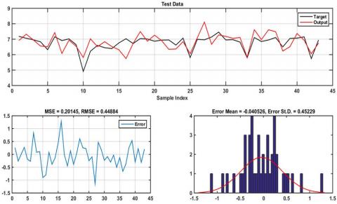
Figure 7. The results of ANFIS-PSO of CR value for testing data
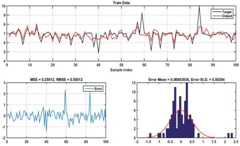
Figure 8. The results of ANFIS-FA of CR value for training data
In the current study, root mean square error (RMSE) and mean square error (MSE) were adopted to evaluate the potency of the proposed metaheurstic algorithm and estimate the CR value along a given set of road links. RMSE and MSE can be calculated as [22, 24]:
fitness function=RMSE $=\sqrt{\frac{\sum_{\mathrm{i}=1}^{\mathrm{n}}\left(\mathrm{X}_{\text {test }}-\mathrm{X}_{\mathrm{obs}}\right)^2}{\mathrm{n}}}$ (26)
$\mathrm{MSE}=\frac{1}{\mathrm{~N}} \sum_{\mathrm{i}=1}^{\mathrm{n}}\left(\mathrm{X}_{\text {test }}-\mathrm{X}_{\mathrm{obs}}\right)^2$ (27)
With, $\mathrm{X}_{\text {test }}$ is the value predicted by ANFIS, $X_{o b s}$ indicates the observed value, and N represents the number of observed data.
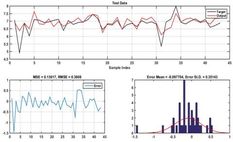
The numerical simulation results of ANFIS based PSO, FA, HBBO and ICA are represented in Figures 6-13 for both testing and training dat.
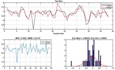
Figures 6-7 represent the results obtained by ANFIS-PSO for both training and testing data, which evidently proves that it provides height accuracy with MSE=0.033, RMSE=0.183 in the training step and MSE=0.201, RMSE=0.448 in testing phase. Plots of desired data against estimated data from the ANFIS-FA model during training and testing are illustrated in Figures 8–9. From the simulation, the minimum training MSE and RMSE was 0.265 and 0.515, while the obtained testing MSE and RMSE was 0.13 and 0.36. It is quite clearly seen that the ANFIS-FA shows a good tracking performance. The simulation results of Figures 10-11 demonstrates that the ANFIS-HBBO fits the desired data accurately and the error distribution acquire a Gaussians distribution with the mean of 0.0008, standard deviation (STD) 0.5 for training data and mean of -0.089, STD of 0.4 during the testing data. Figures 12-13 depicts the response of ANFIS-ICA against the desired CR value, as is evident the predicted data shows a close proximity to the CR value.
Figure 9. The results of ANFIS-FA of CR value for testing data
Figure 10. The results of ANFIS-HBBO of CR value for training data
Figure 11. The results of ANFIS-HBBO of CR value for testing data
Figure 12. The results of ANFIS-ICA of CR value for training data
Figure 13. The results of ANFIS-ICA of CR value for testing data
In this research paper ANFIS model has been successfully designed and simulated with the help of four meta-heuristic approach (PSO, FA, ICA and HBO). The applied approach has been introduced to predict the CR of an accident in road transportation of hazardous material. The proposed technique outperform deterministic approaches in many fields it can adequately treat uncertainties, avoid the inclusion of expert, further examine the criteria that influences the risk value, handle the environment changes of those criteria and it adequately be trained with many optimization algorithm. In other side the given algorithms are capable to provide height accuracy with height dimensional function and bypass local minima's. The simulation results and overall performance comparison concludes that the ANFIS gives height precision and ANFIS-PSO over-perform other technique in the training process, ANFIS-FA provide height performance in testing phase.
It is quite obvious that the RMSE and MSE are less than one in all the predictions, showing an excellent performance, which proves that the implemented techniques is suitable to forecast the CR value. Although the results from proposed hybrid approaches are seemingly good, the comparison in figures 6-13 illustrates the presence of significant differences in the attainable prediction errors. From the figures, the ANFIS model achieved very low average errors (MSE and RMSE) with PSO in the training phase and with FA in testing phase. The combination of fuzzy logic and artificial neural networks coupled with PSO, FA, HBBO and ICA increases its ability to tackle non-linearities in the datasets and its capability to avoid local minima.
[1] Sabar, M., El Hammoumi, M. (2020). Regulatory and institutional context of dangerous goods road transport at the international, African and Moroccan levels. International Journal of Safety and Security Engineering, 10(2): 255-261. https://doi.org/10.18280/ijsse.100213
[2] Zhao, L., Cao, N. (2020). Fuzzy random chance-constrained programming model for the vehicle routing problem of hazardous materials transportation. Symmetry, 12(8): 1208. https://doi.org/10.3390/sym12081208
[3] Pamučar, D., Ljubojević, S., Kostadinović, D., Đorović, B. (2016). Cost and risk aggregation in multi-objective route planning for hazardous materials transportation—A neuro-fuzzy and artificial bee colony approach. Expert Systems with Applications, 65: 1-15. https://doi.org/10.1016/j.eswa.2016.08.024
[4] Men, J., Jiang, P., Xu, H. (2019). A chance constrained programming approach for HazMat capacitated vehicle routing problem in Type-2 fuzzy environment. Journal of Cleaner Production, 237: 117754. https://doi.org/10.1016/j.jclepro.2019.117754
[5] Zhou, L., Guo, C., Cui, Y., Wu, J., Lv, Y., Du, Z. (2020). Characteristics, cause, and severity analysis for hazmat transportation risk management. International Journal of Environmental Research and Public Health, 17(8): 2793.
[6] Derse, O., Göçmen, E. (2021). Transportation mode choice using fault tree analysis and mathematical modeling approach. Journal of Transportation Safety & Security, 13(6): 642-660. https://doi.org/10.1080/19439962.2019.1665600
[7] Chen, J.R., Zhang, M.G., Yu, S.J., Wang, J. (2018). A Bayesian network for the transportation accidents of hazardous materials handling time assessment. Procedia Engineering, 211: 63-69. https://doi.org/10.1016/j.proeng.2017.12.138
[8] Weng, J., Gan, X., Zhang, Z. (2021). A quantitative risk assessment model for evaluating hazmat transportation accident risk. Safety Science, 137: 105198. https://doi.org/10.1016/j.ssci.2021.105198
[9] Ghaleh, S., Omidvari, M., Nassiri, P., Momeni, M., Lavasani, S.M.M. (2019). Pattern of safety risk assessment in road fleet transportation of hazardous materials (oil materials). Safety Science, 116: 1-12. https://doi.org/10.1016/j.ssci.2019.02.039
[10] Mohammadfam, I., Kalatpour, O., Gholamizadeh, K. (2020). Quantitative assessment of safety and health risks in hazmat road transport using a hybrid approach: A case study in tehran. ACS Chemical Health & Safety, 27(4): 240-250. https://doi.org/10.1021/acs.chas.0c00018
[11] Zhang, G., Thai, V.V., Law, A.W.K., Yuen, K.F., Loh, H.S., Zhou, Q. (2020). Quantitative risk assessment of seafarers’ nonfatal injuries due to occupational accidents based on bayesian network modeling. Risk Analysis, 40(1): 8-23. https://doi.org/10.1111/risa.13374
[12] Zhang, Q., Zhuang, Y., Wei, Y., Jiang, H., Yang, H. (2020). Railway safety risk assessment and control optimization method based on FTA-FPN: A case study of Chinese high-speed railway station. Journal of Advanced Transportation, 2020: 1-11. https://doi.org/10.1155/2020/3158468
[13] Bronfman, A., Marianov, V., Paredes-Belmar, G., Lüer-Villagra, A. (2015). The maximin HAZMAT routing problem. European Journal of Operational Research, 241(1): 15-27. http://doi.org/10.1016/j.ejor.2014.08.005
[14] Starčević, S.M., Gošić, A.M. (2014). Methodology for choosing a route for transport of dangerous goods: Case study. Vojnotehnički Glasnik, 62(3): 165-184. http://doi.org/10.5937/vojtehg62-4970
[15] Jang, J.S. (1993). ANFIS: adaptive-network-based fuzzy inference system. IEEE Transactions on Systems, Man, and Cybernetics, 23(3): 665-685. https://doi.org/10.1109/21.256541
[16] Mandal, S., Mahapatra, S.S., Patel, R.K. (2015). Neuro fuzzy approach for arsenic (III) and chromium (VI) removal from water. Journal of Water Process Engineering, 5: 58-75. https://doi.org/10.1016/j.jwpe.2015.01.002
[17] Kennedy, J., Eberhart, R. (1995). Particle swarm optimization. In Proceedings of ICNN'95-International Conference on Neural Networks, 4: 1942-1948. https://doi.org/10.1109/ICNN.1995.488968
[18] Yang, X.H. (2008). Firefly algorithm. Nature-Inspired Metaheuristic Algorithms, 20: 79-90.
[19] Ahmadi, S.A. (2017). Human behavior-based optimization: A novel metaheuristic approach to solve complex optimization problems. Neural Computing and Applications, 28(1): 233-244. https://doi.org/10.1007/s00521-016-2334-4
[20] Golberg, D.E. (1989). Genetic algorithms in search, optimization, and machine learning. Addion Wesley, 1989(102): 36.
[21] Atashpaz-Gargari, E., Lucas, C. (2007). Imperialist competitive algorithm: an algorithm for optimization inspired by imperialistic competition. In 2007 IEEE Congress on Evolutionary Computation, pp. 4661-4667. https://doi.org/10.1109/CEC.2007.4425083
[22] Shirzadi, A., Bui, D.T., Pham, B.T., Solaimani, K., Chapi, K., Kavian, A., Revhaug, I. (2017). Shallow landslide susceptibility assessment using a novel hybrid intelligence approach. Environmental Earth Sciences, 76(2): 1-18. https://doi.org/10.1007/s12665-016-6374-y
[23] Bui, D.T., Pradhan, B., Lofman, O., Revhaug, I., Dick, O.B. (2012). Spatial prediction of landslide hazards in Hoa Binh province (Vietnam): A comparative assessment of the efficacy of evidential belief functions and fuzzy logic models. Catena, 96: 28-40. https://doi.org/10.1016/j.catena.2012.04.001
[24] Bui, D.T., Panahi, M., Shahabi, H., Singh, V.P., Shirzadi, A., Chapi, K., Ahmad, B.B. (2018). Novel hybrid evolutionary algorithms for spatial prediction of floods. Scientific Reports, 8(1): 1-14. https://doi.org/10.1038/s41598-018-33755-7