Amir Majid
© 2021 IIETA. This article is published by IIETA and is licensed under the CC BY 4.0 license (http://creativecommons.org/licenses/by/4.0/).
OPEN ACCESS
The power sharing of PV sets with battery banks in a low voltage distribution network, is optimized with the aim of extending network lifetime. The network lifetime is analyzed using a probabilistic model, in which each PV-battery set has a certain failure probability of supplying power to any load demand center. This probability is assumed to be of normal distribution, that is related to other factors such as power rating, coverage availability, and battery DoD. To extend network lifetime, redundancies in power sharing are removed by activating different groups of PV sets at different times, with durations depending on their joint Gaussian probabilities in supplying the load demands. The contribution of each PV-battery set, is estimated in an intuitive method according to the evaluated probabilities, in which the network is converted into source nodes and load nodes distributed as an ad hoc network, with formulated Gaussian probabilities. An economic load dispatch is then evaluated among the selected PV sets of probabilities higher than a predefined threshold value, to optimize power sharing of the load. A case study of several PV-battery sets supplying several distributed loads, is analyzed and simulated, with formulated joint probabilities. It is found that lifetime is extended by 190% for three PV sets supplying two load centers.
Ad hoc LV network, economic dispatch, gaussian distribution, lifetime extension
Low voltage (LV) power networks are economic means of supplying electrical power when installing low power supplies nearer to the load demands to reduce operating costs as well as infrastructure costs [1]. Eliminating long transmission lines, transformers and switchgear as well as utilizing lower ratings of these units, will avoid higher capital costs as well as operating costs. Examples of LV distributed networks supplying nearby loads, are LV ratings of gas turbine PV sets, diesel PV sets, wind turbines, solar and PV modules [2].
Solar and PV modules, being free energy supplies, are attractive for LV networks, despite the fact, that their power ratings are low. Yet they can be used as supplementary method for supplying part of the network grid load. Banks of batteries are installed to store energy at no-sun times. Proper sizing of PV modules and battery banks are crucial to maintain supplying the daily load demand [3].
The lifetime of PV cells is considerably high, yet the associated batteries suffer from depth of discharge (DoD) constraints. Employing the LV distributed network as an ad hoc network with power supply nodes and load nodes [4], would increase the lifetime of the connected components, as only some units can supply all load centers demands at certain time durations. Hence, redundancies of activating all units at the same time, are avoided [5].
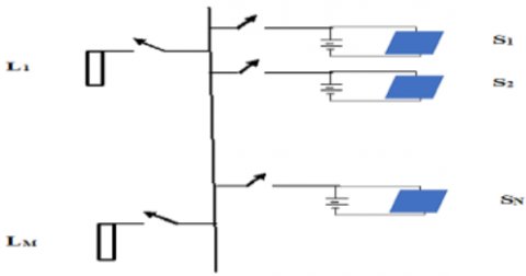
Figure 1 depicts a LV distribution network in which PV modules with battery banks (S1-SN) can be switched on-off depending on the most probable method and least costs for supplying load centers (L1-LM).
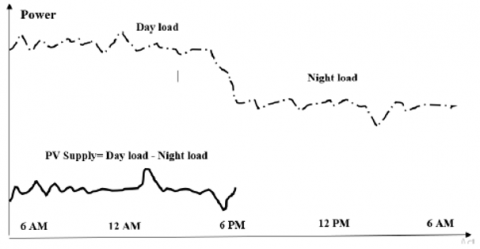
In many cases, domestic and residential load distributions, show that the load demand is higher at nights, in which the difference between night and day load distributions can be supplied by the solar PV sets, as illustrated in Figure 2.
Figure 1. PV sets in a LV distribution network
Figure 2. Typical daily load distribution
A probabilistic model is attempted in which each PV unit, as a source node has a certain coverage failure probability for supplying any load center demand or load node [6]. Failure probability of value 1 indicates no supply coverage. This assumption of source-node to load-node of power supply failure probability, is assumed to be determined from operational and statistical data such as power availability and certainty, distance from supply to load center, operating losses, transmission lines losses, and other running costs. In this work, coverage failure probability is determined basically by the battery depth of discharge (DoD) and power availability of the PV modules proportional to the load demand.
PV set-load coverage problem is to analyze i PV sets (i=1..N), covering j targeted loads (j=1..M), according to power coverage failure probabilities of each PV set node to each load node (gfp), and all PV set nodes to any load node (lfp), by r subsets or groups of sets, with r ϵ [1, k], k=2N-1, i.e.,
$l f p_{j}=\prod_{i} g f p_{i j}$ (1)
and the whole network power coverage failure probability is
$c f p_{r}=1-\prod_{r}\left(1-l f p_{j}\right)$ (2)
with cfpris a power coverage failure probability of all subsets or group of PV sets, which are supplying power to all targeted load zones. To enhance the reliability of the method used, we impose a predefined user-inputted maximum failure probability to be achieved by PV subsets, denoted by α, in which only subsets with entire network failure coverage probabilities less than this value, will be considered for further analysis.
Previous literature shows that algorithms were implemented in wireless networks, such as sensors and actuators networks, that are analogous to distributed PV sets networks, using different methods and algorithms, such as genetic, linear programming, greedy, scheduling techniques, and efficient power sharing [7].
To apply a method for removing redundancies in having all PV sets active all the time, each subset is to be energized in a different time slot that is fraction of the normalized activation period in a cyclic manner, according to an intuitive method, that allocates proportionately time sharing with the coverage failure probabilities.
Lifetime extension is performed as a two folded attempt, namely, time slot activation of each PV set, as well as adjusting PV sets powers in a most economic method. Hence, a dispatch analysis [8] is implemented to determine the economical sharing of generation among each subset’s PV sets.
2.1 PV-battery lifetime extension
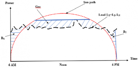
Figure 3 depicts PV generation of electricity following the sun path at a certain location and day of the year. Sizing of the PV modules, and battery banks, is performed according to the availability of solar energy during day times. The system is normally used as a free supplementary power supply.
Figure 3. Load sharing of PV sets and battery banks
It is assumed that night load is supplied by the traditional grid utility, yet day load can be shared with solar PV units incorporated with battery banks that supply power when PV generation is reduced following the sun path, as demonstrated in Figure 2, i.e.,
$G_{P V}=B_{X}+B_{Y}$ (3)
The rating of battery banks, is related with their depth of discharge, while the PV rating is set to be the peak of load distribution waveform that accounts for the difference between day load and night load, as sown in Figure 2, since it is assumed that for domestic and residential applications, day load is normally higher than night load, that is,
$L_{X}=L_{D}-L_{N}$ (4)
We shall use these two constraints to determine the coverage failure probability of each connected PV systems with any load center. The two constraints are namely the PV supply probability, that depends on supply duration of access load, and the battery supply probability, which depends on proportionality of DoD’s with their ratings, as
$\operatorname{Prob}(P V)=1-G_{P V} /\left(12 L_{X}\right)$ (5)
$\operatorname{Prob}(B a t)=B_{X Y} / G_{P V}$ (6)
where, BXY is the larger of BX or BY.
With such as LV networks, it is assumed that frequent switching PV units, is not inadequate and so by letting each subset of PV units, to be active for an allotted time slot, then their lifetimes can be increased, since some PV units with the incorporated battery banks will be inactive during rest of the powering period. Hence, it is required to maximize the extension of lifetime by calculating $\sum_{i=1}^{k} t_{i}$, where tiis the time slot or interval in which one PV units subset may cover all targeted load zones. There are k possible number of PV subsets, that can supply all load demands, with $k=2^{N}-1$, N=number of PV units. It is to be noted that if a PV unit belongs to more than one subset, then the sum of the time intervals in which it is active, cannot be larger than one, since it’s assumed that the normalized lifetime of any component is unity.
For a number of subsets and number of PV units within each subset, time sharing for the activation of PV units can be intuitively estimated in one of 4 methods, i.e., equal or uniform subsets durations with equal PV sets activations, variable subset durations with equal PV units activations, equal subset durations with variable PV units activations, or variable subset durations with variable PV sets activations. No matter which method to be used, lifetime is extended.
Subsets sharing being estimated in terms of the coverage failure probability of whole network, whereas time sharing of each PV sets activated, is according to individual PV set failure probability to cover all load demands. In a study [9], it is found that lifetime can be extended to more than 120%.
2.2 PV-battery joint probability
Each PV set has a certain probability of supplying power to a load in a sustainable manner, that is governed by network individual element components’ probabilities, such as power availability and supply continuity, occurrence of frequent faults, ease of manpower and resources accessibility, etc., that each can be estimated to be having a maximum speculated value according to a normal probability distribution function (PDF) with respect of variation in the mean power coverage from a source node to a load node.
Estimation of the power coverage probability can be evaluated intuitively from knowledge of field and operational statistical databases. It is assumed that the overall probability of all PV sets to one load center, are independent to each other [10], that’s,
Here we shall assume that the individual element of power coverage probability is not uniform, but follows a Gaussian PDF pattern, with an average value, and a covariance.
For a PV set-load network of N PV-sets covering M target load zones, the joint Gaussian pattern [11] is
$F_{X}(x)=\frac{1}{\sqrt{(2 \pi)^{N} \operatorname{det}\left(C_{x x}\right)}} \exp (E)$ (7)
where, $E=-0.5\left(x-\mu_{x}\right)^{T} C_{x x}{ }^{-1}\left(x-\mu_{x}\right)$, µx is an N vector of mean values =[ µ1 µ2 .. µN]T and Cxx is an N x N covariance matrix
$\left[\begin{array}{ccc}\sigma_{1}^{2} & \rho \sigma_{1} \sigma_{2} & \cdots & \rho \sigma_{1} \sigma_{N} \\ \rho \sigma_{1} \sigma_{2} & \sigma_{2}^{2} & & \vdots \\ \rho \sigma_{1} \sigma_{N} & \cdots & & \sigma_{N}^{2}\end{array}\right]$ (8)
It can be deduced that for the two-dimension matrix, the joint PDF is
$f_{X, Y}(x, y)=\frac{1}{2 \pi \sigma_{X} \sigma_{Y} \sqrt{\left(1-\rho^{2}\right)}} \exp (c)$ (9)
where,
$c=\left(\frac{x-\mu_{X}}{\sigma_{X}}\right)^{2}-2 \rho_{X Y}\left(\frac{x-\mu_{X}}{\sigma_{X}}\right)+\left(\frac{x-\mu_{Y}}{\sigma_{Y}}\right)^{2}$ (10)
The relation of joint Gaussian probability of Eq. (9) can be represented symbolically by Matlab platform as,
$f_{X, Y}(x, y)=\frac{5}{12} \frac{\exp \left(-\frac{25}{36} * x^{2}+\frac{5}{18} * x-\frac{5}{18}+\frac{10}{9} * y * x+\frac{5}{18} * y-\frac{25}{36} * y^{2}\right)}{p i}$ (11)
And for a case of multiple joint Gaussian PDF networks, comprising of several PV sets, feeding several load centers, when the coverage probabilities being all mutually uncorrelated, i.e., con(xi,xj)=0, the direct result of this case, is when the off-diagonal elements of the covariance matrix are zero, That’s,
$C V_{X X}=\left[\begin{array}{ccc}\sigma_{1}^{2} & \cdots & 0 \\ \vdots & \ddots & \vdots \\ 0 & \cdots & \sigma_{N}^{2}\end{array}\right]$ (12)
the determinant of which can be evaluated as
$\operatorname{det}\left(C_{X X}\right)=\sigma_{1}^{2} \sigma_{2}^{2} .. \sigma_{N}^{2}$ (13)
and the inverse as,
$C V_{X X}^{-1}=\left[\begin{array}{ccc}\sigma_{1}^{-2} & \cdots & 0 \\ \vdots & \ddots & \vdots \\ 0 & \cdots & \sigma_{N}^{-2}\end{array}\right]$ (14)
The quadratic form that appears in the exponent of the joint Gaussian PDF, E becomes
$\left(x-\mu_{x}\right)^{T} C V_{x x}^{-1}\left(x-\mu_{x}\right)=\sum_{n=1}^{N} \frac{\left(x_{n}-\mu_{n}\right)^{2}}{\sigma_{n}^{2}}$ (15)
It can be deduced that uncorrelated Gaussian random variance are independent, and equal to the product of their marginal PDFs. This concept can be extended to multi-dimensional Gaussian PDF, each with PV set-to-load related parameters, in order to find the overall function.
$\operatorname{Prob}(A \cap B \cap C . .)=\operatorname{Prob}(A) \operatorname{Prob}(B) \operatorname{Prob}(C)..$ (16)
That’s, for Gaussian functions with no correlation, they become independent to each other, which implies that the joint Gaussian PDF is merely the cross multiplication of each marginal PDF.
2.3 Economic load dispatch
Following the evaluation of PV subsets to share supplying all demand loads according to the algorithm of lifetime extension, as well as sharing of each PV unit in the subsets in time slots within a referenced period, we shall next find the optimum economic dispatch of the PV sets activation.
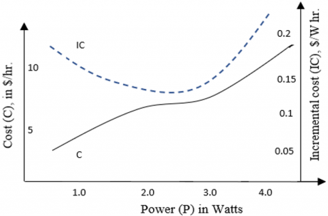
In general, the operating cost Ci of a network is increasing with output power [12]. This cost includes variable costs such as installation, operation and maintenance of battery banks due to DoD, power rectifiers and invertors as well as associated switchgear equipment, and may be represented in a 2nd order parabolic equation, as depicted in Figure 4 for an example [13].
Figure 4. Power cost (C) and incremental cost (IC)
It is required to find PV-battery sets outputs that minimize $C_{T}=\sum_{\mathrm{i}=1}^{\mathrm{N}} \mathrm{C}_{i}$, subject to the equality constraint $P_{T}=P_{1}+P_{2}+. . P_{N}$. The criterion for solving this problem is that all PV sets should operate at equal incremental operating costs [8] as,
$\frac{d C_{1}}{d P_{1}}=\frac{d C_{2}}{d P_{2}}=. .=\frac{d C_{N}}{d P_{N}}=\lambda$ (17)
Inequality constraints can be included too, such as limitations on PV sets output powers, in which each PV set must operate within limits, i.e. Pmin < Pi < Pmax, for i=1..N. So that if one or more PV set reach their limit values, then these PV sets are held at their limits, and the remaining PV sets operate at equal incremental operating cost λ.
We may also impose power loss constraint, such as transmission lines losses, in which the economic dispatch problem can be modified into $P_{T}=P_{1}+P_{2}+\ldots+P_{N}-P_{L}$, where PL represents the losses. Since PL is not constant but depends on the PV outputs, therefore λ in (17) is modified to
$\lambda=\frac{d C_{i}}{d P_{i}}\left(\frac{1}{1-\frac{\partial P_{L}}{\partial P_{i}}}\right)$ (18)
To simplify analysis, we shall ignore this limitation of transmission line losses in this study since we imposed power failure probabilities from PV sets nodes to load nodes.
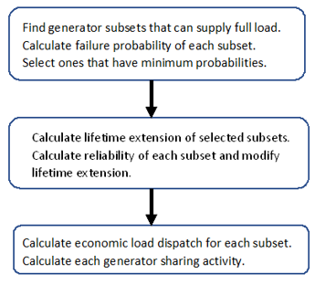
3.1 Algorithm of used method
The procedure steps listed in the Appendix, depicts steps used in the algorithm, namely estimating failure coverage probabilities of PV sets and battery banks, evaluation of the joint Gaussian probability, calculating lifetime extension with the removal of redundancies, as well as contributions of each PV set in sharing total load demand [14].
Initially, failure probabilities of each PV subset that supplies entire load demands is estimated, as there are 2N-1 subsets for N PV sets, according to Eq. (5). Similarly, failure probability of battery bank connected with the PV set, is calculated according to Eq. (6). As it is assumed that these probabilities follow a normal pattern, the joint Gaussian probability is estimated, according to Eq. (20). The estimation technique is not precise, confined or qualitative, yet it can be modified or adjusted by such as field operational and statistical data [15, 16]. Further work maybe needed in future.
Power coverage sharing of each PV subset as well as for each PV set within a subset, are calculated to remove redundancies of energizing all PV units, that put constraints on jeopardizing depth of discharge of batteries. As a result, increasing lifetime of the entire system. Optimum economical dispatch of the operation of the PV network is then analyzed and evaluated according to Eq. (17) and (18).
3.2 Lifetime extension simulation
A case study simulating a network of three PV sets covering two targeted load centers, denoted here as 3G-2L, with values of mean vector and joint covariance matrix for each load as $\mu 1=\left[\begin{array}{lll}0 & 0 & 0\end{array}\right]$, $\mu 2=\left[\begin{array}{lll}1 & 0 & -1\end{array}\right]$, and
$C V_{1}=\left[\begin{array}{ccc}4 & 1 & 2 \\ 1 & 5 & 3 \\ 2 & 3 & 6\end{array}\right] \quad C V_{2}=\left[\begin{array}{ccc}5 & 3 & -1 \\ 3 & 4 & 2 \\ -1 & 2 & 6\end{array}\right]$
for the two loads.
Since there are three PV sets X, Y & Z to cover the entire load demands, there exist seven different PV set combinations or subsets to be studied, according to Eq. (11), by considering variations in the mean or average values of the covered power.
Table 1 shows the joint probabilities of all of these seven combinations for load 1, denoted as F1 and for load 2 as F2, as well as for the total overall load FT. Here, it is considered a variation in the mean power value of Δ=3, whereas, for Tables 2 & 3 are for variation values of Δ=4 and Δ=5 respectively.
Table 1. Joint probabilities of PV sets with random variable variation value of 3
|
|
F1 |
F2 |
FT |
|
X |
0.0028 |
0.0241 |
0.6748e-4 |
|
Y |
0.0060 |
0.0028 |
0.1680e-4 |
|
Z |
0.0096 |
0.0021 |
0.2016e-4 |
|
XY |
0.0070 |
0.0154 |
1.0780e-4 |
|
YZ |
0.0119 |
0.0062 |
0.7378e-4 |
|
XZ |
0.0092 |
0.0037 |
0.3404e-4 |
|
XYZ |
0.0014 |
0.0014 |
0.0196e-4 |
It is seen from Table 1 that combinations {X, XY, YZ} have total probabilities more than a threshold value of 0.5e-4 when mean power variations of Δ=3, whereas for Table 2, the power variation of Δ=4, shows that the combinations {X, Z, XY, YZ} have total probabilities within the same 0.5e-4 threshold value, and Table 3 indicates that combination {X, Z, XY, YZ} are within this same threshold value.
Table 2. Joint probabilities of PV sets with random variable variation value of 4
|
|
F1 |
F2 |
FT |
|
X |
0.0012 |
0.0146 |
0.1752e-4 |
|
Y |
0.0030 |
0.0012 |
0.0360e-4 |
|
Z |
0.0053 |
0.0010 |
0.0530e-4 |
|
XY |
0.0019 |
0.0065 |
0.1235e-4 |
|
YZ |
0.0052 |
0.0020 |
0.1040e-4 |
|
XZ |
0.0032 |
8.0475e-4 |
0.0257e-4 |
|
XYZ |
3.8878e-4 |
0.0014 |
0.0196e-4 |
Table 3. Joint probabilities of PV sets with random variable variation value of 5
|
|
F1 |
F2 |
FT |
|
X |
3.8507e-4 |
0.0073 |
0.0281e-4 |
|
Y |
0.0012 |
3.8507e-4 |
0.0046e-4 |
|
Z |
0.0025 |
4.0371e-4 |
0.0100e-4 |
|
XY |
3.6509e-4 |
0.0021 |
0.0076e-4 |
|
YZ |
0.0018 |
4.593e-4 |
0.0082e-4 |
|
XZ |
8.3695e-4 |
1.1081e-4 |
0.0009e-4 |
|
XYZ |
7.3083e-4 |
0.3943e-4 |
0.0000e-4 |
The above assumption of assigning values of mean vector and joint covariance matrix, is arbitrary and based on probabilities of power coverage of each PV sets, as well as value of battery bank DoD, according to Eq. (16), being independent.
Since, redundancies of the activation of PV sets are to be eliminated, according to the evaluated joint probabilities, only PV subsets {X}, {XY}, and {YZ}, with evaluated load coverage probabilities of {0.6748e-4, 1.0780e-4, 0.7378e-4}, need to be energized, in proportional with these values. These values are based on one of previously studied case. Intuitively, the contribution time of any PV subset CT can be estimated as
$C T_{i}=\frac{\text { Prob }_{i}}{\sum_{i=1}^{k} \text { Prob }_{i}}$ (19)
where, k is number of combinations. So for the subset {X, XY, YZ}, X=27.38%, XY=43.28% and for YZ=29.62%. It can further be deduced that for combination XY, the contribution of X within XY is 80%, hence the total rounded contribution of the three PV sets are: $X=27.38 \%+80 \% \times 43.28 \%=62 \%$,
$\mathrm{Y}=20 \% \times 43.28 \%+45.45 \% \times 29.6 \%=22 \%$, Z=16%.
Table 4 depicts the PV sets power sharing contributions for variations in the mean covered power equal to Δ=3, Δ=4 and Δ=5 respectively.
Table 4. PV sets combinations with random variable variation values 3, 4 and 5
|
Variations of covered power |
GENERATOR |
||
|
X |
Y |
Z |
|
|
variation=3 |
62% |
22% |
16% |
|
variation=4 |
61% |
15% |
24% |
|
variation=5 |
64% |
7% |
29% |
|
Average |
62% |
15% |
23% |
The values of these variations are comparable with the mean and variances of the assumed PDF’s of the three PV sets. We may consider as many variations as inticipated from realistic situations, and the average of these variations is to be used.
As seen from Table 4, PV sets X, Y and Z share 62.3%, 14.6% and 23% respectively of the total operating time, when average variations are imposed. We can conclude from the above calculations, that 190% of the entire PV sets lifetime is saved.
It must be noted, that whereas a threshold value of 0.5e-4, has been selected in the overall joint probability, for Table 1, any other appropriate value can be selected, yet the contributions of PV sets activation, will be changed accordingly. This threshold value depends on many factors, such as limitations on minimum or maximum allowed generated power of PV sets, accuracy of the method used, estimate of the variation of covered power, etc., [17, 18]. Further work may be investigated in selecting this threshold val.
3.3 Economic dispatch simulation
It can be noted from Tables 3, 4 and 5, that the 3 subsets; {X}, {XY} and {YZ} are dominant subsets, in which the two PV sets, X and Z contribute most in the sharing the network energizing time. This is deduced from the average variations of received power as shown in Table 4. Hence, we shall analyze a case study of two PV sets X and Z.
We assume the following operating cost in ȼ/hr. for the two PV sets: C1 = 10x10-2 P1 + 8x10⁻³ P12 and C2 = 8x10⁻² P2 + 9x10⁻³ P22, with the incremental costs: dC1/dP1 = 10x10-2 +16x10-3 P1 and dC2/dP2 = 8x10⁻² +18x10-3 P2.
With dC1/dP1= dC2/dP2 =λ, and simplifying the above, we get $P_{1}=0.53 P_{T}-0.588$, and $P_{T}=P_{T}-P_{1}$, which leads to the value: dC1/dP1= dC2/dP2= 8.47x10 -3PT + 9.44x10⁻³.
We shall as well impose limitation constraints on the two PV sets as: 1 MW ≤ P1 ≤ 9 MW, and 4 MW ≤ P2 ≤ 15 MW
Table 5 summarizes PV set power distribution among the two PV sets for a load demand varying from 5 MW to 20 MW, together with total operating costs.
Table 5. Load dispatch for minimum operation
|
P MW |
P1 MW |
P2 MW |
dC/dP $/MWhr |
CT $/hr |
C1+2 $/hr |
C2+1 $/hr |
|
5 |
1 |
4 |
1.160 |
02.840 |
07.000 |
06.440 |
|
6 |
2 |
4 |
1.320 |
04.080 |
08.880 |
08.050 |
|
7 |
3 |
4 |
1.480 |
05.480 |
10.920 |
09.840 |
|
8 |
3.652 |
4.348 |
0.772 |
06.847 |
13.120 |
11.810 |
|
9 |
4.182 |
4.818 |
0.857 |
08.056 |
15.480 |
13.960 |
|
10 |
4.712 |
5.288 |
0.941 |
09.428 |
16.370 |
16.290 |
|
11 |
5.242 |
5.758 |
1.026 |
10.885 |
17.440 |
18.800 |
|
12 |
5.772 |
6.228 |
1.111 |
12.426 |
18.690 |
21.490 |
|
13 |
6.302 |
6.698 |
1.196 |
14.053 |
20.120 |
24.360 |
|
14 |
9 |
5 |
1.700 |
18.130 |
21.730 |
27.410 |
|
15 |
9 |
6 |
1.880 |
19.200 |
3.520 |
30.640 |
|
16 |
9 |
7 |
2.060 |
20.450 |
25.490 |
34.050 |
|
17 |
9 |
8 |
2.240 |
21.880 |
27.640 |
37.450 |
|
18 |
9 |
9 |
2.420 |
23.490 |
29.970 |
42.450 |
|
19 |
9 |
10 |
2.600 |
25.280 |
32.480 |
49.050 |
|
20 |
9 |
11 |
2.780 |
27.250 |
35.170 |
57.250 |
Note: C1+2: PV set 1 power is varied initially until limit, when PV set 2 takes over, C2+1: PV set 2 power is varied initially until limit, when PV set 1 takes over.
Note that due to the lower limit of P2 =4 MW, we make λ= dC1/dP1 and hence P1=PT-4MW, whereas for P1 reaching 9MW, it was held constant at 9MW, with P2=PT-P1, with λ= dC2/dP2.
As shown in the above table, the average for the economic operating cost = 14.361 $/hr, whereas for the non-economic operation cases, we have two cases:
For calculating C1+2 (i.e., PV set 1 is varied initially until limit, when PV set 2 takes over), we assign the values of P1 and P2 as
P1 = [5 6 7 8 9 9 9 9 9 9 9 9 9 9 9 9]
P2 = [0 0 0 0 0 1 2 3 4 5 6 7 8 9 10 11]
that is, unit 1 starts supplying power until reaching maximum limitation, when the second unit takes over to supply a maximum load demand of 20 MW. It is found that the average cost value =20.251 $/hr. Note that unit 2 is idle since unit can satisfy load demand up to 9 W, when the second unit takes over.
Whereas for calculating C2+1 (i.e., (i.e., PV set 2 power is varied initially until limit, when PV set 1 takes over), we assign the values of P2 and P1 as
P2 = [4 5 6 7 8 9 10 11 12 13 14 15 15 15 15 15]
P1 = [1 1 1 1 1 1 1 1 1 1 1 1 2 3 4 5]
that is, unit 2 starts supplying power until reaching maximum limitation, when the unit 1 takes over to supply a remaining maximum load demand of 20 MW. It is found that the average cost value =25.584 $/hr. Note that initially unit 1 supplies 1 MW to accomplish the minimum load demand of 5 MW.
It can be deduced that with economic operation, costs are reduced by 40% with C1+2, and 78% with C2+1. This case study can be extended to cases of more than two PV sets with an implementation of a computer algorithm.
A method is used to extend the lifetime of a LV network, powered by a number of PV-battery bank sets that supply a supplementary load, by removing redundancies of activating all PV sets at the same time. In a case study of 3 PV sets supplying two load centers, the lifetime is increased by 190%.
A novel algorithm is implemented to calculate each PV set contribution, to be proportional to an estimated probability of supplying demand of several load centers. The evaluation of probabilities of PV sets availability and battery DoD, are based on the daily load distribution and sun path, in such a manner that PV modules may charge the battery banks adequately, and supply the supplementary day load. As there are 2N-1 groups for N sets, the joint Gaussian probabilities of all possible activated groups or subsets of PV sets are evaluated.
It is demonstrated that the removal of redundancies depends on the amount of variations in the mean values of the supplied power by any subset, being a random variable. Adequate values of 3 variations are assumed for the most dominant subsets and an average is used in the evaluation of the total joint PDF, that is used for removing PV sets redundancies.
The analysis is demonstrated in a case study of 3 PV sets operating within 7 different subsets to supply the demand of 2 load centers in a LV distributed network, with given PV set-load power coverage probabilities.
For the same case study, an economic dispatch analysis is performed to find the optimum power sharing among the PV sets, according to PV sets power cost and incremental cost values with constraints on their supplied power limits.
|
gfp |
PV set-load nodes failure probability |
|
lfp |
failure probability of all PV sets to a load |
|
cfp |
subset coverage failure probability |
|
GPV |
PV generation |
|
B |
battery energy |
|
k |
PV set subsets |
|
L |
load distribution |
|
Prob |
probability |
|
t |
time slot |
|
F |
joint Gaussian vector |
|
F |
probability function distribution |
|
CV |
covarince matrix |
|
X |
unit X |
|
Y |
unit Y |
|
Z |
unit Z |
|
P |
power |
|
C |
cost |
|
IC |
incremental cost |
|
CT |
time sharing contribution |
|
Greek symbols |
|
|
α |
failure coverage assigned value |
|
σ |
standard deviation |
|
λ |
cost function |
|
Δ |
variations in mean power |
|
ρ |
covarience |
|
Subscripts |
|
|
i, j |
indices |
|
N |
number of units |
|
r |
subset |
Procedural steps performed in this study
[1] Torquato, R., Ricciardi, T.R., Salles, D., Barbosa, T., Costa, H.F. (2012). Review of international guides for the interconnection of distributed generation into low voltage distribution networks. IEEE Power and Energy Society General Meeting, San Diego, CA, USA. https://doi.org/10.1109/PESGM.2012.6345519
[2] Boyle, G., Everett, B., Ramage, J. (2003). Transmission, distribution and running the system. Energy Systems and Sustainability, UK, Oxford University Press, 371-381.
[3] He, J., Ji, S.L., Pan, Y., Li, Y.S. (2014). Reliable and energy efficient target coverage for wireless Sensor networks. Tsinghua Science & Technology, 16(5): 464-474. https://doi.org/10.1016/S1007-0214(11)70066-9
[4] Majid, A. (2015). Maximizing ad hoc network lifetime using coverage perturbation relaxation algorithm, WARSE International Journal of Wireless Communication and Network Technology, 4(6): 77-83.
[5] Duncan Glover, J., Sarma, M.S. (2002). Power system control. Power System Analysis and Design, 3rd Ed., USA, Brooks/Cole, 525-540.
[6] Miller, S.L., Childers, D. (2012). The Gaussian random variable. Probability and Random Processes, 2nd Ed., USA, Academic Press (Elsevier}, 71-78.
[7] Zhang, H., Wang, H.Y., Feng, H.C. (2009). A distributed optimum algorithm target coverage in wireless sensor networks. IEEE Asia-Pacific Conference on Information Proceedings, 2: 144-147. https://doi.org/10.1109/APCIP.2009.172
[8] Freris, L., Infield, D. (2008). Optimum economic dispatch. Renewable Energy in Power Systems, USA, Wiley, 200-205.
[9] Miller, S.L., Childers, D. (2012). Gaussian random variables in multiple dimensions. Probability and Random Processes, A book, 2nd Ed., USA, Academic Press (Elsevier}, 249-252, ISBN 9780123869814.
[10] Miller, S.L. Childers, D. (2012). Gaussian random variables in multiple dimensions. Probability and Random Processes, 2nd Ed., USA, Academic Press (Elsevier}, 249-252.
[11] Stark, H., Woods, J. (2002). The multidimensional Gaussian law. Probability and Random Process with Applications to Signal Processing, USA, Prentice Hall, 269-277.
[12] Hodge, B. (2010). System economics and operation. Alternative Energy Systems and Applications, USA, John Wiley, 277-295.
[13] Majid, A. (2020). Lifetime Extension with Economic Load Dispatch of Low Voltage Ad Hoc Distributed Networks. Paper Accepted for Oral Session to the 8th International Conference on Electrical Energy and Networks ICEEN2020, Singapore.
[14] Verheggen, L., Ferdinand, R., Moser, A. (2016). Planning of low voltage networks considering distributed generation and geographical constraints. IEEE International Energy Conference, (ENERGYCON). http://dx.doi.org/10.1109/ENERGYCON.2016.7514042
[15] Sarajlić, D., Rehtanz, C. (2019). Low voltage benchmark distribution network models based on publicly available data. IEEE PES Innovative Smart Grid Technologies Europe (ISGT-Europe). http://dx.doi.org/10.1109/ISGTEurope.2019.8905726
[16] Kumar, D.S., Savier, J.S. (2017). Impact analysis of distributed generation integration on distribution network considering smart grid scenario. IEEE Region 10 Symposium (TENSYMP). http://dx.doi.org/10.1109/TENCONSpring.2017.8070023
[17] Caire, R., Retiere, N., Morin, E., Fontela, M., Hadjsaid, N. (2013). Voltage management of distributed generation in distribution networks. IEEE Power Engineering Society General Meeting. http://dx.doi.org/10.1109/PES.2003.1267183
[18] Everett, B. (2004). Casting energy. Energy Systems and Sustainability, Oxford press, UK, 477-512.