Mohamed Azzazen*![]() | Salah Boukraa
| Salah Boukraa![]()
© 2023 IIETA. This article is published by IIETA and is licensed under the CC BY 4.0 license (http://creativecommons.org/licenses/by/4.0/).
OPEN ACCESS
It is generally assumed, sometimes implicitly, that the exploding gas cloud is uniform and homogeneous. However, in practice, the cloud often results from an accidental release of a chemical substance into the air, leading to a non-uniform gas mixture and, therefore, gradients of concentration of pressure or temperature. These gradients correspond to distributions of the degree of reactivity and, consequently, to a greater or lesser ability to react. In addition, they influence the consequences of the explosion. This study aims to investigate the behaviour of these gradients in the case of explosions in a reactive, non-uniform and confined environment. The phenomena of diffusion, combustion, and flame propagation of heterogeneous mixtures within closed chambers are carried out through numerical simulations. Moreover, a comparative study with previously published works is developed and presented to validate our results.
temperature gradient, pressure gradient, gas mixture, combustion, flame propagation, diffusion
Combustion is a chemical reaction that proceeds in localized regions, so-called flame. The flame is characterized by the apparition of temperature and pressure gradients and the variation of products and reactants concentrations. The process of diffusion is one of the principal complex physical phenomena strongly coupled, allowing the description of non-premixed combustion, also known as diffusion combustion [1-4].
Studying heterogeneity phenomena in combustion is one of the principal means to control energy conversion. Various industrial systems are the subject of applications, particularly the production of thermal energy (boilers or domestic and industrial furnaces), electricity (thermal power plants), or also applications related to transport (automobile and aeronautical engines, rocket engines). Nearly 90% of the world's energy needs are supplied by combustion phenomena which consist of many physical and chemical processes to be studied [5, 6]. Combustion of inhomogeneous mixtures requires, in particular, the determination of the pressure field and the determination of the flame velocity and its propagation. Therefore, these parameters have a critical interest [7-9].
In this work, we are particularly interested in the problems related to the degree of reactivity distribution in a reactive and confined environment and the difficulties related to considering heterogeneities. In addition, we are interested in the analytical modelling and the numerical resolution of Fick's law. Furthermore, a case of combustion diffusion was investigated. The equations that govern this phenomenon are complex and coupled. Many studies have focused on non-premixed combustion modelling, and computational fluid dynamics (CFD) progress proposes a lot of models, including in three most numerous approaches [10-14]:
In this study, a model based on LES approach is applied. Various numerical and semi-empirical techniques were used to calculate the various physical and chemical parameters to determine the temperature and pressure evolution during combustion, the species production rate and the flame velocity produced by a chemical reaction of propane and oxygen [5-12]. The simulations are carried out under the CFD ANSYS software. They are conducted to visualize the flame propagation and its velocity, the pressure and temperature distributions.
Our study is part of the research of solutions that minimize or limit the industrial risks of detonation while reducing polluting gas emissions produced by the energy transformers. This approach makes it possible to establish the best conditions for using a non-polluting gas mixture in thermal machines.
The paper is structured into five different sections. After an introduction, Section 2 presents the experimental setup used in the detonation laboratory. Section 3 is devoted to mathematical modelling and presenting the Navier-Stokes equations that describe the reactive flows. Section 4 discusses the obtained results. Finally, conclusions are presented in Section 5.
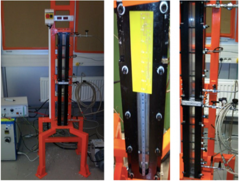
Figure 1 shows our experimental configuration. It consists of a tube with two equal chambers of the same volume separated by a membrane (valve). Both chambers have the same total pressure Pt=1 atm and are at a uniform temperature T=298.170 K. They contain two mixtures, M1 and M2, of different compositions and mass fractions, introduced into the combustion zone using priming at the bottom of the tube after a diffusion delay. The experiment is carried out according to two cases presented in Table 1.
The present specific experimental tool concerns the control of the formation of heterogeneous mixtures and forms a new set of associated flame propagation and acceleration mechanisms for these mixtures.
Our proposed structure is an experimental novelty. It is adapted to the data of a transparent straight tube with a closed square cross-section, chosen for the following reasons: it favours the visualization of the flame and allows obtaining of various measures through sensors. It also allows excellent control of the concentration gradients by favouring, with some precautions, the mixing mechanisms by molecular diffusion.
Figure 1. Experimental configuration
Table 1. Reagent distribution
|
Mixtures |
||
|
Case 1 |
M1 M2 |
100% O2 100% C3H8 |
|
Case 2 |
M1 M2 |
100% C3H8 100% O2 |
The operation is based on improving technical features, including the experimental setup, to develop a wide variety of experiments. These experiments are characterized by visualizing the flame of a moving and stopping sequence with control using sensors and photodiodes connected to digital oscilloscopes. This is achieved after an optimal choice of all features.
The various operations include control, recording and visualization of the flame with the help of the proposed and implemented circuits and modules, allowing obtaining and exploiting of results. The intermediate phases are the initiation of the experimental operation in different setups and the recording after elaborating on different stages of the experiment.
The units used for this experimental installation's design, operation and specifications are composed of cooling and auxiliary elements, which constitute the components of this circuit and assembly elements. In addition, the above units are connected and equipped with sensors and a digital oscilloscope. These are used to produce controls and digital command of flames, objects of experiments processed at the input of the automatic installations and during the execution of all stages.
The experimental installation proposed for the various experiments is suitable for all kinds of experimental conditions. The installation is attached to a base held by a structure, which also supports the column of the transparent, straight tube module, which is the subject of the experimental studies. A frame is an assembly of steel beams of 5 cm2 cross-section welded together, supporting the tube and rising to a suitable height. It keeps the tube vertical at a reasonable height from the ground, as presented in Figure 2.
Inside this structure, the elements for the different experiments are implanted and fixed (pump motor, spark plug).
The results of the elaborated experiments are obtained with the help of a digital oscilloscope, photodiodes (Figure 2(b)) placed along the section on the left side of the installation, and two pressure sensors placed in the middle of each section (Figure 2(c)). Notice that the different units and elements are cooled by cooling equipment.
(a) Total installation (b) Photodiodes (c) Section and column
Figure 2. Overview of the experimental setup
A leakage test is required before the experiment is carried out by using compressed air with the help of a motor pump. Then, the system is emptied into the chamber of the experimental installation with an open valve that separates the two sections under investigation. After that, the system is ready for a new experiment: filling the two sections in a separate state with different gases up to a pressure of one bar on both sides and the valve is closed to isolate each section from the others.
After a spark production, the flame, the object of evaluation, which propagates in a tube of 1 m long in the presence of heterogeneous propane-oxygen of gas mixtures, will be formed by molecular diffusion through a flap valve. This valve ensures full communication between the sections without any blocking effects in the open position.
Combustion phenomena involve several different scientific disciplines, essentially: chemistry, thermodynamics, and fluid mechanics. It is, therefore, essential to use an appropriate combustion model. Depending on the model chosen, the non-premixing problems are governed by fluid mechanics equations coupled with those of thermochemistry [15]. The equations governing the behaviour of this model are conservation of mass, conservation of momentum, energy and propane-oxygen concentration for a Newtonian compressible fluid, so-called the Navier-Stokes equations. In the absence of external volume forces, the generalization of these equations for a reactive flow leads to the following system of equations:
3.1 Conservation of mass equations
The total mass balance, as well as the balance of each species, are written as:
$\frac{\partial \rho}{\partial t}+\frac{\partial \rho}{\partial x_j}\left(\rho u_j\right)=0$ (1)
$\frac{\partial\left(\rho Y_k\right)}{\partial t}+\frac{\partial\left(\rho u_j Y_k\right)}{\partial x_j}=-\frac{\partial J_j^k}{\partial x_j}+\dot{\omega}_k \quad$ for $k=1 \ldots N$ (2)
where, $u_j$ is the 'ith' component of the velocity vector, Yk is the mass fraction of species k, $\dot{\omega}_k$ is the reaction rate and $J_j^k$ represents the diffusive flux of species given by the following expression:
$J_j^k=-\rho D \frac{\partial\left(Y_k\right)}{\partial x_j}$ (3)
where, Dk is the diffusion coefficient.
The theory of gas diffusion in another at low-pressure results from the resolution of the Boltzmann equation. It was developed independently by Levermore [16]. They came up with the following equation:
$D_{A B}=1.8583 .10^{-7} \frac{T^{3 / 2}}{P M_{A B}^{1 / 2} \quad\sigma_{A B}^2 \quad\Omega_D}\left[m^2 / s\right]$ (4)
where, T is the ambient temperature, M is the molecular masses of the gases considered, P is the ambient pressure, $\sigma_{A B}^2$ is the Lennard-Jones characteristic length and ΩD is the Lennard-Jones energy parameter.
3.2 Conservation of momentum
$\frac{\partial\left(\rho u_j\right)}{\partial t}+\frac{\partial\left(\rho u_i u_j\right)}{\partial x_j}=-\frac{\partial P}{\partial x_i}+\frac{\partial \tau_{i j}}{\partial x_j} \quad i=1,2,3$ (5)
where, P is the pressure such that $p=R_0 T \sum \frac{\rho_k}{w_k}$, ρk and wk are the density and molar mass of species k. $\tau_{i j}$ is the viscous stress tensor given by Newton's law:
$\tau_{i j}=\mu\left(\frac{\partial u_i}{\partial x_j}+\frac{\partial u_j}{\partial x_i}\right)-\frac{2 \mu}{3}\left(\frac{\partial u_k}{\partial x_k}\right) \delta_{i j}$ (6)
where, μ is the dynamic viscosity of the mixture, and δij is the Kronecker delta.
3.3 Energy equation
The total energy is the sum of the internal energy, the kinetic energy, and the chemical energy. Let (E=ei+ec) be the total non-chemical energy, then we have:
$\frac{\partial \rho \mathrm{E}}{\partial t}+\frac{\partial \rho u_i \mathrm{E}}{\partial x_i}=\dot{\omega}_T-\frac{\partial q_j}{\partial x_j}+\frac{\partial\left(\tau_{i j}-p\right) u_i}{\partial x_j}$ (7)
where, $\dot{\omega}_T$ is the heat release rate, $\frac{\partial q_j}{\partial x_j}$ is the heat flux and $\frac{\partial\left(\tau_{i j}-p\right) u_i}{\partial x_j}$ is the strength of the viscous and pressure forces.
We note that the introduced thermochemical equations allow us to model the interaction between fluid mechanics and combustion and the chemical reactions between the different components of the gas mixture. The properties of combustion result from the combined action of chemical (rapid production of heat and reactive chemical species), physical (transport, diffusion), material and heat displacement processes [4]. These properties can be characterized using different parameters: the nature and number of reactants, the mode of introducing reactants, and the gas flow regime in the reaction medium [2, 3].
3.4 Conservation equation for chemical species
The overall chemical reaction of combustion of a hydrocarbon (CnHm) can be written:
$\begin{aligned} & C_n H_m+\left(n+\frac{m}{4}\right)\left(O_2+3.76 \mathrm{~N}_2\right) \rightarrow n \mathrm{CO}_2+ \frac{m}{2} \mathrm{H}_2 \mathrm{O}+\left(n+\frac{m}{4}\right) 3.76 N_2+Q\left[m^2 / s\right]\end{aligned}$ (8)
where, Q is the amount of heat released by stoichiometric combustion.
On the other hand, non-stoichiometric combustion is characterized by other parameters, such as the dilution ratio 'α' and the excess air coefficient '$\phi$'.
The resolution of these equations allows knowing at any point and at any time the composition, the temperature and the pressure of the mixture of the reactive gas. The thermochemical state of the mixture is determined by two parameters, the mass fraction of the fuel and the fraction of the mixture. Suppose the walls of the studied systems are considered adiabatic and impermeable to species. In this case, we can define the fraction of the mixture, noted '$\xi$' [5], which represents both the evolution of enthalpy 'h' and mass fraction of any species, we have:
$\xi=\frac{\left(Y-Y_1\right)}{\left(Y-Y_2\right)}+\frac{\left(h-h_1\right)}{\left(h_2-h_1\right)}$ (9)
where, the indices subscripts characterize the oxidizer and the fuel, respectively. This expression states that $\xi=0$ in the pure oxidant and $\xi=1$ in the pure fuel. It should be recalled that Fick's second law expresses the transient regime where we assume $\frac{\partial \rho}{\partial t} \neq 0$.
The variation of the concentration with time is then defined by the equation:
$\frac{\partial \rho}{\partial t}=-D_{A B}\left(\frac{\partial^2 \rho}{\partial x^2}+\frac{\partial^2 \rho}{\partial y^2}+\frac{\partial^2 \rho}{\partial z^2}\right)$ (10)
Diffusion is a spontaneous, irreversible, and inescapable phenomenon that results in the migration of chemical species in a medium. We observe a displacement of constituents leading to equilibrium under thermal agitation and concentration difference. This phenomenon is governed by a law stated by Adolf Fick and bears his name [7].
In what follows, we are initially interested in solving Fick's law to calculate the mixture's concentration. We note that this concentration is a function of time and space. Moreover, the results obtained by simulation are used experimentally and then used in a second step as parameters in the Navier-Stokes equations presented above.
The obtained solution describes the combustion mechanism through the flame propagation, velocity, and pressure increase when the flame crosses these gradients, knowing that the boundary conditions are:
$\left\{\begin{array}{l}\left.\frac{\partial C}{\partial x}\right|_{x=0}=0 \\ \left.\frac{\partial C}{\partial x}\right|_{x=1}=0\end{array}\right.$ (11)
and the following initial condition:
$C(x, 0)= \begin{cases}C 1 & \text { si } x \in[0,0.5[ \\ C 2 & \text { si } x \in] 0.5,1]\end{cases}$ (12)
4.1 Dissemination
A numerical simulation of the influence of heterogeneity on flame propagation is carried out after verifying the compatibility of the evolution of the concentrations in the space-time domain of our numerical simulation results with the experimental results by taking into account various compositions of mixtures. This simulation enabled us to identify the parameters (pressure, speed velocity) that increase or decrease deflagration-detonation transition risk. The results below show the species' concentration evolution for different delays. In addition, a representation of the velocity is made to highlight the behaviour of the mixture during diffusion.
4.1.1 Compatibility of diffusion times with Fick’s law
Our simulation considers that the valve between the two sections is open at the initial state. The upper part of the tube contains a mixture of 20% by volume of methane/air, whereas only air is present in the lower part of the tube. We used the evolution of the percentage of oxygen (O2) in the tube to check the compatibility of mixing times with Fick's law. The comparison between numerical and experimental results presented in the study [5] for the case of methane/air mixing at a fixed axial abscissa for different times presents a negligible difference.
The numerical results are obtained by solving Fick's law. On the other hand, a measuring device, such as an oxygen meter, is necessary to read the oxygen concentration (O2) during the experiments.
The initial decrease and difference in the initial concentrations are due to the fact that the initial concentration of oxygen (O2) in the cell of the oxygen meter is higher than that in the tube. The initial decrease, which we observe with Fick's law, corresponds to two simultaneous phenomena. Indeed, methane diffuses in the cell, and oxygen concentration decreases to reach the oxygen rate in the tube. However, we cannot observe these phenomena in our simulation since we must consider how a measuring device could influence species diffusion.
A comparison between the experimental results implemented by Daubech [5] and our calculations is made through data presented in Table 2. It is noticeable that a good qualitative agreement is reached regarding the diffusion of species. Furthermore, this equation is remarkably verified by calculating the maximum relative error (E=1.58%) for the measured quantity.
Table 2. Compatibility of diffusion times with Fick's law
|
Time |
O2 |
O2 Exp |
Time |
O2 |
O2 Exp |
|
0 |
0.1700 |
0.1760 |
12000 |
0.17561 |
0.17349 |
|
600 |
0.16843 |
0.1728 |
12600 |
0.17604 |
0.1740 |
|
1800 |
0.16848 |
0.16973 |
13800 |
0.17685 |
0.17467 |
|
2400 |
0.1686 |
0.1692 |
14400 |
0.17723 |
0.17493 |
|
3000 |
0.16881 |
0.16893 |
15000 |
0.17761 |
0.17547 |
|
3600 |
0.16911 |
0.16893 |
15600 |
0.17797 |
0.17573 |
|
4200 |
0.16948 |
0.16893 |
16200 |
0.17832 |
0.1760 |
|
4800 |
0.16991 |
0.1692 |
16800 |
0.17866 |
0.17627 |
|
5400 |
0.17036 |
0.16947 |
17400 |
0.17899 |
0.17634 |
|
6000 |
0.17086 |
0.16979 |
18000 |
0.17932 |
0.17653 |
|
6600 |
0.17134 |
0.17026 |
18600 |
0.17965 |
0.17741 |
|
7200 |
0.17184 |
0.17067 |
19200 |
0.17991 |
0.17748 |
|
7800 |
0.17233 |
0.1708 |
19800 |
0.1802 |
0.17821 |
|
8400 |
0.17283 |
0.1712 |
20400 |
0.18075 |
0.1784 |
|
9600 |
0.1738 |
0.172 |
21600 |
0.18127 |
0.1788 |
|
10200 |
0.17427 |
0.17227 |
22200 |
0.18151 |
0.17906 |
|
10800 |
0.17423 |
0.1728 |
22800 |
0.18175 |
0.17918 |
|
11400 |
0.175 |
0.173 |
23400 |
0.1819 |
0.1797 |
4.1.2 The influence of density on diffusion
To investigate the influence of density on diffusion, we examined the mixtures listed in Table 1. A series of simulations with propane-oxygen proportions for combustion in a confined volume are carried out, and the main results are presented in the latest sections.
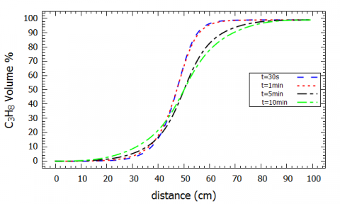
The distribution of oxygen (O2) is a function of the distance along the central axis of the square-section tube (Distance x=0 m at the bottom and x=1 m at the top of the tube) and diffusion time. These results allow us to identify the impact of density on diffusion. At different times (30 sec, 1 min, 5 min, 10 min), we plotted the molecular diffusion, and we sought to know the influence of the density of the mixtures on the diffusion and the critical diffusion time intervals. For this purpose, we modelled two different cases:
Case 1: the lower part of the tube is filled with propane (C3H8), while the upper part is filled with oxygen (O2).
This means that the densest species is located at the bottom of the tube. We have taken measurements at different times. The Figure 3 (Figure 3(a), (b) and (c)) shows the distribution of the two mixtures along the tube for different diffusion times for this case. We can notice that the diffusion time is equal to 240 min.
(a) Diffusion of O2
(b) Diffusion of C3H8
(c) The diffusion time
Figure 3. Diffusion of O2, C3H8 species from case 1
(a) Diffusion of C3H8
(b) The diffusion time
Figure 4. Diffusion of O2, C3H8 species from case 2
Case 2: the lower part of the tube is filled with oxygen (O2) while the upper part is filled with propane (C3H8).
This means that the densest species is located at the top of the tube (M1 100% C3H8, M2 100% O2). Figure 4 (Figure 4(a), (b)) shows the distribution of the two mixtures along the tube for different diffusion times. In this case, we can notice that the diffusion time equals 210 min, therefore, if we increment the simulation time as examples to 230 min and 260 min, we observe that the obtained curves are constant values with the same level obtained at 210 min. Comparing with the obtained results from case 1 (M1: 100% O2, M2: 100% C3H8), where the diffusion time was 240 min, it should be noted that the diffusion time becomes lower.
The different obtained results show that molecular diffusion is a slow phenomenon. Figure 4(c) shows that the diffusion rate is important in other regions where the concentration gradient is more significant, even if it is very low. We underline that these different simulations aim to simulate the combustion by a layer of an inhomogeneous mixture.
For all treated cases with the two configurations, the obtained results show that the time of homogenization is essential, allowing us to analyse the diffusion phenomenon of the chemical species, particularly those that form an explosive mixture. Moreover, the analysis helps predict the risk of combustion and the deflagration-detonation transition.
4.1.3 Influence of gravity on diffusion
To study the influence of gravity on the diffusion phenomenon, the mass fraction values for the same element are reversed. The choice of this method is justified by the Brownian motion that characterizes the diffusion phenomenon and the difficulty in predicting the behaviour of the gas elements involved.
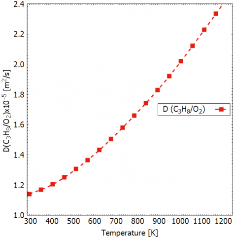
In this situation, Figure 5 shows that the influence of gravity is weak and even negligible. This observation can be explained by other phenomena (inter-molecular interactions) that overcome the force of gravity, which logically accelerates diffusion. We can see that the diffusion is essentially due to a strong concentration gradient and thermal agitation. Even if the influence of temperature does not appear explicitly in the Fick equation, it is introduced in the diffusion coefficient.
Figure 6, which represents the diffusion coefficient evolution with temperature, shows an exponential variation of this parameter.
Eq. (4), which results from the solution of the Boltzmann equation, was developed independently by Bobylev [17] and allowed the effect of temperature on the diffusion coefficient to be evaluated as a thermally activated quantity. Indeed, all the calculations are conducted based on the atomic theory of diffusion. According to the Arrhenius law, the increase in temperature implies the increase of the diffusion coefficient, which means the acceleration of the diffusion phenomenon due to thermal agitation.
Figure 5. Influence of gravity
Figure 6. Evolution of the diffusion coefficient
4.2 Combustion simulation
The use of propane (C3H8) raises many questions, particularly concerning the problems associated with its safety during transport or storage, for example. From this point of view, the physical process of propane (C3H8) combustion in a confined environment must be controlled so that the obtained results (temperature, pressure) should not exceed the limits set by technological considerations. The combustion chamber considered in this study has the same geometry as the one used for the diffusion phenomenon. The purpose is to determine the evolution of the flame propagation, its velocity and the total pressure of the combustion, which is the effect most often requested.
Indeed, the improvement of the mixture makes it possible to minimize many problems, such as the instability of the combustion and the emission of pollutants, while improving the output.
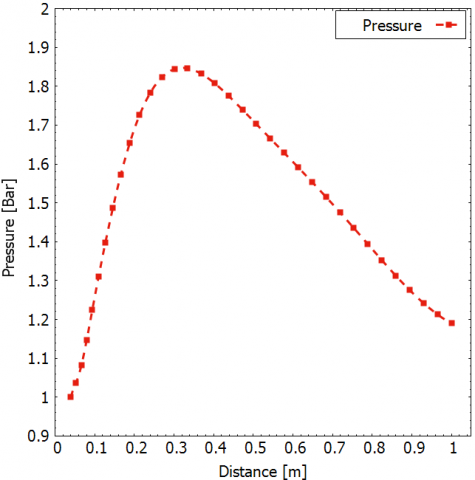
The adiabatic temperature obtained by the numerical simulation of the flame is equal to 2100 K, considering the radiation effect. Figures 7 and 8 show the temperature evolution and the total pressure for each tube position. A significant increase in temperature is observed as a function of the distance, this is mainly due to the nature of the gases mixture and to the fact that the walls are adiabatic. However, the pressure increases from the bottom to the mid-height of the tube then decreases in its upper part, this depends on many factors, particularly due to the decrease in the mixture concentration and the geometry of the confined medium.
Experimental measurements initiated by Daubech [5] allowed us to obtain the Figure 9, where we present the flame propagation evolution in our tube. We collected a database of 1500 pictures taken at time intervals of 1ms. In Figure 9, we observe that initially the flame is located at the bottom part of the tube then propagates up to the top until the distance of 1m. Using these measures, we can estimate the flame velocity evolution as function of distance from the bottom this is illustrated in the Figure 10, where we compare the experimental results with those obtained numerically.
The flame velocities obtained by our simulations are compared in Figure 10 with those obtained experimentally from the video recordings. In the two cases, the obtained results show that combustion takes place in the tube axis direction and that its speed initially increases then decreases with distance from the bottom. It appears that the numerically predicted flame velocities are slightly overestimated, this being mainly due to the fact that we did not consider the heat losses through the walls because they are considered adiabatic. However, it is noted that even the experimental results may suffer from a lack of precision.
Figure 7. Evolution of the combustion temperature
Figure 8. Evolution of the combustion pressure
Figure 9. Evolution of the flame propagation
Figure 10. Evolution of the flame propagation velocity
It can be deduced that there is a combustion wave at the front, characterized by a decrease in pressure and density together with an acceleration of the gases through the reaction zone, where the reactants are transformed into burnt products.
This paper provides a highly accurate verification of the compatibility of Fick's Law, combustion and flame propagation of a heterogeneous mixture in closed combustion chambers. This study aimed to use numerical simulation to have a more realistic view by considering the different processes involved. The numerical simulation of diffusion and combustion of a gas mixture of propane and oxygen in a confined tube is governed by the conservation laws coupled with the law of perfect gases. The flow parameters and the concentrations of the different chemical species are calculated step by step as a function of time until the equilibrium state is reached. It has been noticed that the higher the velocity, the higher the temperature, and the faster the diffusion is exerted. Thus, the rate of production increases and consequently, the velocity of the flame increases, while the pressure increases until all the reagents are consumed, followed by a reduction in pressure.
The obtained results allow us to better understand the actual situation after comparing the theory with the experiments in the proposed physical model, especially combustion.
The authors would like to express their special thanks and sincere gratitude to the deceased Pr. YOUBI Zine-eddine, who conceived the idea of this work.
|
$D_k$ |
Diffusion coefficient |
|
$J_j^k$ |
Diffusive flux of species |
|
h |
Enthalpy |
|
M |
Molecular masses of the gases considered |
|
P |
Ambient pressure |
|
$Q$ |
Heat released by stoichiometric combustion |
|
T |
Ambient temperature |
|
$u_i$ |
ith component of the velocity vector |
|
$w_k$ |
Molar mass of species k |
|
$Y_k$ |
Mass fraction of species k |
|
Greek symbols |
|
|
$\alpha$ |
Dilution ratio |
|
$\delta_{i j}$ |
Kronecker delta |
|
$\xi$ |
Fraction of the mixture |
|
$\rho_k$ |
Density of species |
|
$\mu$ |
Dynamic viscosity of the mixture |
|
$\sigma_{A B}^2$ |
Lennard-Jones characteristic length |
|
$\tau_{i j}$ |
Viscous stress tensor |
|
ϕ |
Excess air coefficient |
|
$\Omega_D$ |
Lennard-Jones energy parameter |
|
$\dot{\omega}_T$ |
Heat release rate |
|
$\dot{\omega}_k$ |
Reaction rate |
|
Subscripts |
|
|
k |
Species index |
[1] Kuo, K., Acharya, R. (2012). Fundamentals of Turbulent and Multiphase Combustion. John Wiley & Sons. https://doi.org/10.1002/9781118107683
[2] Chung, K. (2006). Law Combustion Physics. Cambridge University Press, New-York. https://doi.org/10.1017/CBO9780511754517
[3] Thierry, P., Denis, V. (2005). Theoretical and Numerical Combustion. 2nd Edition, Edwards, Pa, USA. https://doi.org/10.1016/j.combustflame.2005.11.002
[4] Michael, L. (2008). Introduction to Physics and Chemistry of Combustion. Springer, Germany.
[5] Daubech, J. (2008). Contribution to the study of effects of heterogeneity of a gaseous premixed on flame propagation in a closed tube. Doctoral thesis, University of Orleans, USA.
[6] Sochet, I., Guelon, F., Gillard, P. (2002). Deflagrations of non-uniform mixtures: A first experimental approach. In Journal de Physique IV (Proceedings), 12(7): 273-279. https://doi.org/10.1051/jp4:20020294
[7] Gülen, S. (2019). Combustion in Gas Turbines for Electric Power Generation. Cambridge University Press, Cambridge, pp. 308-361. https://doi.org/10.1017/9781108241625
[8] Bauwens, C.R., Chaffee, J., Dorofeev, S.B. (2011). Vented explosion overpressures from combustion of hydrogen and hydrocarbon mixtures. International Journal of Hydrogen Energy, 36(3): 2329-2336. https://doi.org/10.1016/j.ijhydene.2010.04.005
[9] Bennoud, S., Azzazen, M. (2017). Simulation of viscous incompressible flow through a conduit with isothermal walls. In International Workshop on the Complex Turbulent Flows (IWCTF2017), Tangier, Morocco, November, pp. 27-28.
[10] Jaffe, R., Taylor, W. (2018). Internal Combustion Engines, In the Physics of Energy. Cambridge University Press, Cambridge, pp. 203-218. https://doi.org/10.1017/9781139061292
[11] Djemoui, L., Redjem, H. (2017). Numerical study of the swirl direction effect at the turbulent diffusion flame characteristics. International Journal of Heat and Technology, 35(3): 520-528. https://doi.org/10.18280/ijht.350308
[12] Azzazen, M., Youbi, Z., Bennoud, S. (2018). Simulation and analysis of diffusion Phenomenon of separated gases Mixtures in a confined tube. Journal of Research in Engineering and Applied Sciences, 3(2).
[13] Crank, J. (1975). The matimatics of diffusion. Clarendon press, Oxford.
[14] Sengissen, A.X., Poinsot, T.J., Van Kampen, J.F., Kok, J.B. (2007). Response of a swirled non-premixed burner to fuel flow rate modulation. In Complex Effects in Large Eddy Simulations, pp. 337-351. https://doi.org/10.1007/978-3-540-34234-2_24
[15] Ouali, S., Bentebbiche, A.H., Belmrabet, T. (2016). Numerical simulation of swirl and methane equivalence ratio effects on premixed turbulent flames and NOx apparitions. Journal of Applied Fluid Mechanics, 9(2): 987-998. https://doi.org/10.18869/acadpub.jafm.68.225.22603
[16] Levermore, C.D. (1979). Chapman--Enskog approach to flux-limited diffusion theory (No. UCID--18229). California Univ.
[17] Bobylev, A.V.E. (1982). The chapman-enskog and grad methods for solving the boltzmann equation. In Akademiia Nauk SSSR Doklady, 262(1): 71-75.