Michał Ryms*![]() | Grzegorz J. Kwiatkowski
| Grzegorz J. Kwiatkowski![]() | Witold s.M. Lewandowski
| Witold s.M. Lewandowski![]()
© 2023 IIETA. This article is published by IIETA and is licensed under the CC BY 4.0 license (http://creativecommons.org/licenses/by/4.0/).
OPEN ACCESS
On the basis of theoretical considerations of convective-radiative heat transfer, a relationship was developed enabling the total convective and radiative heat flux QC+R emitted from any object at tw and its surroundings at t∞ to be calculated from known values of the surface temperature of such an object, i.e., the known temperature difference Δt=tw - t∞ and average air temperature Tav. This relationship is applied to thermal imaging cameras with the aim of developing appropriate software to enhance their measurement capabilities. They can then be used not only for monitoring and measuring temperature, local overheating, heat losses through insulation materials, thermal bridges, constructional defects, moisture, etc., but also for measuring the heat losses from any object, such walls and buildings. This empirical relationship includes constants relating to the object itself, such as its characteristic dimension l, surface area A, emissivity ε and temperature parameters, which depend on tw, t∞, Δt and Tav and on the physical properties of air. Experimental validation of the proposed relationship, performed for two values of the surface emissivity ε, showing the discrepancies ΔQC+R=1.75% (for ε=0.884) and 4.85% (for ε=0.932), has confirmed its correctness and its practicability.
convective-radiative heat transfer, infrared camera, experiments, empirical equation, vertical plate
Heat transfer in air is a complex mechanism involving both convection and radiation. Despite this mutual coexistence, these two means of heat transfer are usually considered separately, and the results obtained for either of them, though most often for convection, described by Newton's equation, are corrected by subtracting the radiant heat flux calculated with the Stefan-Boltzmann equation. On the other hand, when determining heat losses, the calculated radiative heat loss flux is added to the measured convective heat flux. To determine the convective heat flux, it is necessary to know the heat transfer coefficient α, the dimensions l and b of the object under consideration and its surface temperature tw, as well as the ambient air temperature in the undisturbed area t∞. In addition, for the radiant flux the temperature of the surrounding walls tot ≈ t∞ and the surface emissivity ε are also required: this latter quantity should be measured, assumed, or be taken from a set of tables that assign their values to typical surfaces (polished copper, brick, plaster, wood, etc.) [1, 2].
At lower temperatures, convection becomes more important and is of great interest to researchers, even though it involves a much higher level of complexity. This emerges from its physical description, which in the case of free convection requires three conjugate partial differential equations (continuity, Navier-Stokes and Fourier-Kirchhoff), the mathematical methods of solving them, and carrying out the relevant experimentation. These difficulties, far from discouraging researchers, have inspired them to study convection even more intensively. At the same time, the only reward they could count on was scientific satisfaction, because industry was not interested in this low-intensity mode of heat transfer. Times and attitudes have changed, however: the primary aim nowadays is to conserve energy, for example, by limiting heat losses, mainly caused by free convection, especially in the construction, energy and metallurgy industries.
At higher temperatures, radiative heat transfer is more important, for the description of which the Planck, Wien, Stefan-Boltzmann and other equations are necessary [3, 4]. In external heat transfer and for simple spatial configurations, especially at low temperatures, radiation can be described only by the Stefan-Boltzmann equation, but its practical use is troublesome. To determine the radiative heat flux from this equation, it is not enough to know the temperatures of the heating surface tw and the surroundings t∞, and the emissivity ε. One also needs to know the temperature of surrounding objects, as well as the humidity and pressure of the air. In the case of internal heat transfer, however, e.g. in heat exchangers, engine cylinder channels or combustion chambers, when the areas of a heated surface Aw and its surroundings A∞ optically interact with each other or take place in optically active media, any considerations of radiation must take into account not only the Stefan-Boltzmann equation, but Kirchhoff’s and Lambert’s laws [5] as well, with which the equivalent emissivity factor εw-∞ and the configuration factor φ=Aw / A∞ can be determined. If Aw and A∞ are parallel, then εw-∞=1 / (1 /εw + 1/ε∞ - 1), and φ=1 [6]; but when Aw is inside A∞ (Aw << A∞), then εw-∞ ≈ εw=ε [7]. Many studies have addressed various configurations of radiative heat transfer surfaces, for example [7-9].
In order to eliminate the effects of radiation in experimental convection studies, some researchers took various approaches, performing experiments in water [10-13], glycerine [14-16] or other liquids like ethylene glycol [17], in which radiation does occur but is much smaller than convection in water (assumption QR=0). Others used polished copper or aluminium plates [18-21] assuming that when ε=0, QR is also equal to 0. The remainder calculated the radiative flux from the Stefan-Boltzmann equation for given values of ε and subtracted it from the heating power of the tested surfaces.
The following convective-radiation studies of heat transfer in a confined space are of interest: the numerical examination of the impact of solar radiation on the conversion of heat transfer from conduction to convection in a three-dimensional (3D) shallow wedge [22], and an investigation, likewise numerical, of the influence of the absorbing-emitting-scattering effect in a two-dimensional (2D) square cavity on convective-radiative heat transfer [23]. Similar problems were studied in a partitioned rectangular enclosure with semi-transparent walls [24], in a cavity with a porous horizontal layer [25], in a side open cavity [26], and also with regard to heat transfer by conduction in the study [27]. An interesting numerical study examining coupled natural convection and surface radiation through an open fracture in a solid wall facing a reservoir containing isothermal quiescent air was reported in the study [28]. A similar study of coupled free convection and radiative heat transfer in a cavity containing an isothermal vertical plate and filled with carbon dioxide or nitrogen was carried out using holographic interferometry [29]. Another numerical study using a participating medium (like carbon dioxide and water vapour) in the channel between two vertical parallel plates was reported in the study [30]. An experimental study of free convection and radiative heat transfer in air inside rectangular closed cavities of different aspect ratio with two vertical active walls (hot and cold) was described in the study [6]. The results of experimental studies of heat exchange in the channel between two symmetrically heated isothermal vertical walls using a thermal imaging camera, in which the contribution of radiation was limited by the polished surfaces of aluminium plates, were given in the studies [31, 32]. In paper [33] the relationship between radiation and convection from a vertical flat plate was interferometrically and numerically (with the FLUENT programme) investigated. The influence of its emissivity and internal heat conduction were also taken into consideration in it.
Numerical and theoretical considerations of convective-radiative heat exchange inside square and rectangular enclosures using the commercial software FLUENT 6.3 and Dimensional Analysis were given in the study [34]. The influence of radiation on laminar convective heat transfer determined in optically active media was numerically tested using the Rosseland approximation [35], and with reference to an isothermal vertical plate in the studies [36-42].
Determination of the specific heat of a vertical plate material and the emissivity of its surface with the use of transient cooling of the solid system consisting in convective-radiative cooling in the air, in the temperature range t=42 – 142℃ and Ra=2.106 - 2.107, was described in papers [43, 44]. Experimental studies of convective-radiative heat transfer from a horizontal cylinder were described in the study [45] and from an isothermal vertical slender cylinder in [46], and different cases that can be found also in the studies [46-48]. The same problem, but theoretically using a similarity solution in relation to the vertical plate, was investigated and described in the studies [49-52]. The interaction of convection with radiation for a plate inclined at a small angle to the horizontal was analysed using the appropriate transformation and then solving the resulting local non-similarity equations numerically [53]. The solution of dimensionless boundary-layer equations of second-order interactions between radiation and free laminar convection from a vertical, black and isothermal plate to the surrounding grey gas was given in the studies [54, 55]. The effect of radiation on free convection was investigated experimentally in the corner formed by a horizontal plate and a vertical fin of height 30, 50 and 70 mm coated with paints of different colours to change the emissivity from 0.05 to 0.85 [56].
Clearly, there is a growing demand for research results relating, among other things, to combined convective-radiative heat exchange in construction, industry and in numerous technological problems, including internal combustion engines, furnace design, nuclear reactor safety, fluidized bed pyrolysis, heat exchangers, solar collectors and photo- and biochemical reactors. These entities are more interested in the magnitude of the heat flux supplied or emitted from a real heat exchange surface than in the heat transfer mechanisms, the participation of convection and radiation in them, the simplifying assumptions made, the experimental procedures etc. The response to this heightened interest in applications of overall convective and radiative heat transfer can be found in papers dealing with heat losses in construction [57-62] and from the housings of industrial devices (motors, pumps, exchangers) [63], and the heat fluxes transferred within specific devices, such as baking ovens [64], internal combustion engine cylinders [65] or glass furnaces [66, 67].
As mentioned above, convection and radiation have usually been considerated separately. But in the case of air, they always coexist and can interact to varying extents, depending on the temperature. The proportion of heat transfer by radiation is higher than by convection and increases as the temperature of the heating surface rises. The study of the interactions of these two heat transfer mechanisms and the search for the possibility of their joint mathematical description in the form of a single empirical equation is the subject of this paper.
2.1 Heat transfer from heated surfaces in air
The density of heat loss from a building, which is the sum of radiation and convection losses qc+R, depends mainly on the temperature difference between the heat transfer surface tw and the ambient temperature t∞ (1). These are not only direct losses through the walls of the building, but also indirect losses through non-residential spaces (staircases, attic and cellars) as shown in the diagram in Figure 1. The mechanism of heat losses from rooms, through walls and ceiling, is connected with convective and radiative heat transfer. From the basement, on the other hand, these losses occur by conduction to the foundations and then to the ground.
Since the temperature difference (tw,in - tground) as well as the thermal conductivity of the foundations have small values, according to Fourier's law this heat loss flux by conduction was neglected qloss,floor ≈ 0, and further consideration was focused on the relevant convective qc and radiative qr partial heat loss fluxes and the total one qc+R in generalized terms: for tw, t∞ and the vertical surface. The obtained relations for other configurations of planar (horizontal, oblique), cylindrical or conical surfaces can be corrected by substituting the relevant CC and n constants for these configurations in the Nusselt-Rayleigh criterion relationships (1 - 5).
Figure 1. Types of heat loss fluxes in a model of a building with an indication of how convective heat fluxes can be directly measured, using thermal imaging camera with a grid [19, 68]
During heating or cooling in air, the temperature difference between a heated surface tw and the surroundings t∞ causes heat to be exchanged by convection (according to Newton's law, this is proportional to the heat transfer coefficient αC), and by radiation (according to the Stefan-Boltzmann theory, this is proportional to the coefficient αR). The total heat flux qc+R can be written as:
$\begin{aligned} q_{C+R}=q_C+q_R= & \alpha_C \cdot \Delta t+\sigma \cdot \varepsilon \cdot\left(T_w^4-T_{\infty}^4\right)= \alpha_{C+R} \cdot \Delta t\end{aligned}$ (1)
where:
$\alpha_C=\frac{\lambda}{l} \cdot N u_C=\frac{\lambda}{l} \cdot C_C \cdot R a^n$, (2)
And similarly
$\alpha_{C+R}=\frac{1}{l} \cdot N u_{C+R}=\frac{1}{l} \cdot C_{C+R} \cdot R a^n$, (3)
Substituting (2) and (3) in (1) gives:
$\frac{\lambda}{l} \cdot C_C \cdot R a^n+\frac{\sigma \cdot \varepsilon}{\Delta t} \cdot\left(T_w^4-T_{\infty}^4\right)=\frac{\lambda}{l} \cdot C_{C+R} \cdot R a^n$ , (4)
And then
$C_{C+R}=C_C+\frac{\sigma \cdot \varepsilon \cdot l}{\lambda \cdot \Delta t \cdot R a^n} \cdot\left(T_w^4-T_{\infty}^4\right)$. (5)
Analysis of Eq. (5) suggests the following cases:
CC values are known from the literature, where they are given in the form of the dependence of Nusselt and Rayleigh numbers obtained from experimental, theoretical and numerical research:
$N u_{\mathrm{c}}=C_{\mathrm{C}} \cdot R a^{\mathrm{n}}$. (6)
The value of CC+R can be determined from the measured heating power q and the heat loss fluxes qstr, as:
$\alpha_{C+R} \cdot \Delta t=q_{C+R}=q-q_{s t r}$, (7)
$C_{C+R}=\frac{Q-Q_{\text {loss }}}{A \cdot \Delta t}=\frac{U \cdot I \cdot l}{A \cdot \lambda \cdot \Delta t \cdot R a^n}$ (8)
For electric heating with a current power Q=U ∙ I, heat transfer area A, characteristic linear dimension l, and when the heat flux is transferred in its entirety to the heated medium (qstr=0).
The emissivity ε of a heated surface is known or can be determined, e.g., with a thermal imaging camera; nonetheless, its value is encumbered with a certain error [69, 70].
Any combination of the three above cases.
2.2 Vertical heated plate
Further considerations of the coexisting mechanisms of heat exchange in the air, i.e., natural convection and radiation, were carried out on the longest tested and best known configuration of the heated surface, i.e. The vertical heated plate. Until recently, the results of theoretical, experimental and numerical research obtained for this were the most frequently published in the scientific literature on free convection, so this configuration of the heated surface is the most representative for validating the correctness of the considerations discussed in this paper.
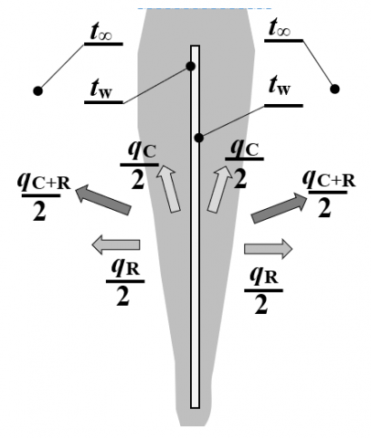
Figure 2. Draft scheme of a thin, double-sided, heated isothermal vertical plate
In the case of electric heating, the heating power can be written as Q=U . I, and in the case of a double-sided vertical plate of width b, height h and area A=2.b.h, the heat energy flux qc+R transferred to the environment consisting, according to Figure 2 and Eq. (1), of two convective qc/2 and two radiative qr/2 fluxes, is proportional to the equivalent (convective-radiative) heat transfer coefficient αC+R, according to the relationship:
$q_{C+R}=\alpha_{C+R} \cdot \Delta t=\frac{Q-Q_{\text {loss }}}{A}=\frac{U \cdot I-Q_{\text {loss }}}{A}$. (9)
Assuming for a thin, double-sided plate that the heat loss Qloss=0 [71], the total heat transfer coefficient αC+R and the Nusselt number Nuc+R can be written as:
$\alpha_{C+R}=\frac{U \cdot I}{A \cdot \Delta t}=\frac{U \cdot I}{2 \cdot b \cdot h \cdot \Delta t}$, (10)
$N u_{C+R}=\frac{\alpha_{C+R} \quad \cdot h}{\lambda}=\frac{U \cdot I}{2 b \cdot \lambda \cdot \Lambda t}$ (11)
From the Nusselt-Rayleigh criterion dependence, analogous to (6) and (2), but for a vertical plate where n=1/4,
$N u_{\mathrm{C}+\mathrm{R}}=C \mathrm{C}+\mathrm{R} \cdot R a^{1 / 4}$, (12)
The constant CC+R, described in detail by (5), can be calculated for specific temperature conditions, determined by the Rayleigh number (16):
$C_{C+R}=\frac{N u_{C+R}}{R a^{1 / 4}}$. (13)
With the results of experimental tests, in the form of known values of tw, t∞, U, I, b, h for temperature conditions (Δt, tav=(tw + t∞)/2), the physical properties of air (β, λ, ν and a), and then Nuc+R, Ra and CC+R can be calculated:
$\frac{N u_{C+R}}{R a^{1 / 4}}=\frac{U \cdot I}{2 b \cdot \lambda \cdot \Delta t \cdot R a^{1 / 4}}=C_{C+R} \quad$. (14)
2.2.1 The case where the heat flux is known
In industry, construction and agriculture (breeding, greenhouse crops), where the lowest possible costs of production or exploitation have to be balanced against high energy costs, technical and economic information on flux values and the amount of heat transferred in technological or operational processes is the most important. Without this information, it is hard to take responsible decisions, manage energy optimally and economically, and reduce costs.
When electrical energy is converted into thermal energy, information on the power of heating or cooling devices and the amount of heat energy they transfer can be obtained by direct measurement of the electrical heating power Q=U.I, taking into account the efficiency of conversion, and their operation time $\tau$. In the case of other energy carriers, e.g., heating or cooling media, to determine the amount of transferred thermal energy, the temperature drop tin - tout of the medium and its mass flow rate M have to be known. In the case of steam heating, the measure is the amount of condensate or the decrease in the enthalpy of the heating steam, etc.
In this situation, the value of CC+R and the heat exchange mechanisms are of secondary importance to the user. Nevertheless, a knowledge of CC+R, calculated from a known value of qc+R, may be useful for analysing other cases of convective heat transfer in air. For this purpose, after rearranging Eq. (8), one obtains:
$\begin{aligned} Q_{C+R}=\frac{U \cdot I}{A}=\alpha_{C+R} \cdot \Delta t & =\frac{\lambda}{h} \cdot N u_{C+R} \cdot \Delta t=\frac{\lambda}{h} \cdot C_{C+R} \cdot R a^{\frac{1}{4}} \cdot \Delta t\end{aligned}$, (15)
$C_{C+R}=\frac{U \cdot I \cdot h}{A \cdot \lambda \cdot \Delta t \cdot R a^{1 / 4}}=\frac{U \cdot I}{2 \cdot b \cdot \lambda \cdot\left(T_W-T_{\infty}\right)} \cdot R a^{-1 / 4}$. (16)
The values of CC+R obtained for specific cases and the heating powers, temperatures, physical properties of air and Ra measured for them, can be used to determine qc+R and QC+R in other heating or cooling systems, where their direct measurement is impossible. These cases are discussed in the next section.
2.2.2 The case where the heat flux and power are not known
It is not always possible to directly measure the heat flux qc+R transferred by the heating medium. This applies, for example, to the heating of spaces with heat pumps, solar collectors, air heaters, as well as heat losses from buildings, cooling of electronic systems, etc. In these cases, to determine the power and amount of transferred heat, it is necessary to know the values of the coefficients CC+R or CC and CR according to the Nusselt-Rayleigh criteria, which can be used to determine the power Q and the heat flux q=Q/A transferred from the heating device to the environment.
With a known (literature) or experimentally determined value of CC+R, the heat transfer flux from surface A can be calculated from (15) as follows:
$q_{C+R}=\frac{\lambda}{h} \cdot C_{C+R} \cdot \Delta t \cdot R a^{1 / 4}$, (17)
$Q_{C+R}=q_{C+R} \cdot A=2 \cdot b \cdot \lambda \cdot C_{C+R} \cdot \Delta t \cdot R a^{1 / 4}$. (18)
If the heated or cooled object consists not only of a single double-sided heated vertical plate, but also of i- such plates or vertical pipes with a diameter d, then the area should be appropriately corrected in formula (18). A=2.b.h.i or A=2.π.d.h.i should be substituted for A =2.b.h, and if such an object contains horizontal components, e.g., a horizontal plate, cuboid or pipe, then the appropriate characteristic linear dimension l and exponent n for Ra should be used in addition.
The value of CC+R can also be determined from Eq. (5), if one knows the literature values of the convective coefficient CC and the calculated radiative heat flux.
The coefficient CC for an isothermal vertical plate has historically taken the following example values: CC=Nu/Ra1/4=0.571 [72],=0.560 [73],=0.540 [74]. In the paper [75] a total of 25 plates of this type were analysed, giving an average value of CC,av=Nu/Ra0.252=0.550. This value, however, is based on the unusual exponent n for a vertical plate that is inconvenient to use, especially when comparing the results. In [71], the coefficients CC and n in the Nusselt-Rayleigh relationship were converted for the assumed values of Ra=106, 7, 8, 9 from n=0.252 to n=0.250, and the following new relationships were obtained:
$\begin{gathered}N u_{\mathrm{c}, \mathrm{av}}=0.550 \cdot R a^{0.252},=0.565 \cdot R a^{0.25}\left(R a=10^6\right), =0.573 \cdot R a^{0.25}\left(R a=10^9\right)\end{gathered}$ (19)
$N u_c=0.569 \cdot R a^{0.25}\left(R a=10^6-10^9\right)[71]$ (20)
This dependence differs from that given in the study [52] (CC=0.555) by only 2.5% and is therefore used later in this paper.
Knowledge of the second part of Eq. (5), i.e., the radiative heat flux, requires the emissivity of the radiator surface ε to be known or measured in addition to the temperatures Tw and T∞. Taking into account both components of the heat flux (convection and radiation), the following relationship can be obtained:
$C_{C+R}=0.569+\frac{\sigma \cdot \varepsilon \cdot l}{\lambda \cdot \Delta t \cdot R a^n} \cdot\left(T_w^4-T_{\infty}^4\right)$ (21)
In technical issues, the most important thing is to know the values of αC+R and the heat transfer flux qc+R, which can be calculated from Eq. (21) based on Eqns. (2), (3) and (4):
$\alpha_{C+R}=\frac{\lambda}{l} \cdot 0.569 \cdot R a^{\frac{1}{4}}+\frac{\sigma \cdot \varepsilon}{\Delta t} \cdot\left(T_w^4-T_{\infty}^4\right)$ (22)
$\begin{array}{r}q_{C+R}=\alpha_{C+R} \cdot \Delta t=\frac{\lambda}{l} \cdot 0.569 \cdot \Delta t \cdot R a^{\frac{1}{4}}+ \sigma \cdot \varepsilon \cdot\left(T_w^4-T_{\infty}^4\right) .\end{array}$. (23)
3.1 Simulation calculations CC+R=f(tw, Δt, l, ε)
Simulation calculations, as well as theoretical, numerical and experimental considerations, require the knowledge or assumption of the temperatures of the heated surface (tw, Tw=tw+273.15), the undisturbed area (t∞, T∞=t∞+273.15), the difference between them Δt=ΔT=tw –t∞ and the average air temperature Tav=(Tw+T∞)/2, for which its physical properties a, cp, β, λ, μ, ρ, ν should be determined. These properties are now available online; in the past, they had to be read from tables, such as [1, 76].
3.1.1 Calculation of the physical properties of air
For the purposes of this work, based on the study [77], the following formulas were derived for calculating the physical properties of air for a given temperature Tav in the range 120 ≤ Tav ≤ 480 K [77]:
β =1/Tav [1/K], or β=7.17643∙10-13 . Tav4 – + 2.76969∙10-10 . Tav3 + 5.36690∙10-8 . Tav2 – + 1.29663∙10-5 . Tav + 3.65078∙10-3 [1/K], R2=0.9998, (24)
a=-7.76593∙10-14 . Tav3 + 1.10718∙10-10 . Tav2 + 8.70331∙10-8 . Tav + 1.3323∙10-5 [m2/s], R2=0.9999, (25)
ν=-1.60765∙10-13 . Tav3 + 1.77128∙10-10. Tav2 + 1.25673∙10-7 . Tav + 1.85135∙10-5 [m2/s], R2=0.9999, (26)
λ=3.13755∙10-11 . Tav3 – 4.27648∙10-8 . Tav2 + 7.70091∙10-5 . Tav + 2.4048∙10-2 [W/(m∙K)], R2=0.9999. (27)
In order to perform simulation calculations of heat transfer in air, the following values were assumed: heated surface temperatures tw=90, 80, 70, 60, 50, 40, 30 and 20℃ and the temperature difference Δt=tw – t∞=5, 10, 15, 20, 40 and 60 K, the combination of which determined the temperature of the undisturbed area t∞ and the average air temperature tav=(tw + t∞)/2.
3.1.2 Introduction of thermodynamic and thermo-emission functions
By introducing the function B1, which determines the thermodynamic properties of air, and B2, related to its thermo-emission, Eq. (21) can be converted into the form:
$\begin{array}{r}C_{C+R}=C_C+C_R=C_C+\frac{\sigma \cdot \varepsilon \cdot l \cdot\left(T_w^4-T_{\infty}^4\right)}{\lambda \cdot\left(T_w-T_{\infty}\right) \cdot R a^{1 / 4}}=C_C+B 1 \cdot B 2 \cdot l^{1 / 4} \cdot \varepsilon\end{array}$, (28)
where:
$B 1=\frac{1}{\lambda \cdot\left(\frac{g \cdot \beta \cdot \Delta t}{\gamma \cdot a}\right)^{\frac{1}{4}}}, \mathrm{~m}^{7 / 4 \cdot \mathrm{K} / \mathrm{W}}$, (29)
$B 2=\frac{\sigma \cdot\left(T_w^4-T_{\infty}^4\right)}{\Delta t}, \mathrm{~W} /\left(\mathrm{m}^2 \mathrm{~K}\right)$, (30)
$R a=\left(\frac{l^{3 / 4}}{\lambda \cdot R 1}\right)^4=\frac{g \cdot \beta \cdot \Delta t \cdot l^3}{v \cdot a}$. (31)
Convective heat transfer, especially in fluids not accompanied by radiation, is more difficult to study experimentally, but it is easier to understand and obtain reliable and reproducible results in the form of CC=Nu/Ran. It is simpler to conduct research in air, especially when a surface is heated electrically, but the inconclusive influence of radiation complicates the interpretation of the results. Perhaps by determining the effect of temperature, separately on the functions B1 and B2 and on their product B1·B2, it will be easier to describe convective-radiative heat transfer and obtain more reliable results.
The measurement uncertainties of the values taken from table data [1, 71, 76-78], was assumed at the level of the last significant digit in the data source. For a temperature measurement the accuracy of ±0.1℃ was assumed, but for the temperature differences, according with the study [71], the calculations permit an accuracy of ±0.05 K to be specified. The maximum relative uncertainties of Ra and CC+R, derived from Eqns. (31) and (21) are: δRamax=± 4.7% and δCC+R max=± 8.5%. In order to preserve the clarity of the presentation the uncertainty of measurement in relation to the maximum relative uncertainty δCmax are only be given in the following investigation. A detailed analysis of the measurement uncertainties related to this consideration can be found in ref. [71].
Table 1. Calculated values of B1 and B2 for given values of tw, t∞ and l
|
Temperatures |
Physical properties of air |
B1 (Figure 3.a) |
B2 (Figure 3.b) |
B1.B2 (Figure 4) |
||||||||||
|
tw |
t∞ |
t,av |
∆t |
λ . 10-2 |
b . 10-3 |
a.10-5 |
n.10-5 |
(29) |
(35) |
(30) |
(33) |
(34) |
(35) |
(36) |
|
℃ |
℃ |
℃ |
K |
W/m.K |
1/K |
m2/s |
m2/s |
m7/4K/W |
W/(m2K) |
1/m1/4 |
||||
|
90 |
85 |
87.5 |
5 |
3.0439 |
2.7843 |
3.0758 |
2.1734 |
0.2748 |
0.2768 |
10.640 |
10.7426 |
2.9239 |
2.9735 |
2.9779 |
|
80 |
75 |
77.5 |
5 |
2.9746 |
2.8656 |
2.9242 |
2.0697 |
0.2723 |
0.2744 |
9.7797 |
9.7945 |
2.6632 |
2.6875 |
2.6923 |
|
70 |
65 |
67.5 |
5 |
2.9042 |
2.9501 |
2.7754 |
1.9678 |
0.2699 |
0.2720 |
8.9667 |
8.9302 |
2.4199 |
2.4287 |
2.4341 |
|
60 |
55 |
57.5 |
5 |
2.8330 |
3.0380 |
2.6295 |
1.8679 |
0.2675 |
0.2696 |
8.2000 |
8.1421 |
2.1931 |
2.1948 |
2.2007 |
|
50 |
45 |
47.5 |
5 |
2.7607 |
3.1300 |
2.4865 |
1.7699 |
0.2650 |
0.2671 |
7.4783 |
7.4236 |
1.9820 |
1.9832 |
1.9896 |
|
40 |
35 |
37.5 |
5 |
2.6875 |
3.2269 |
2.3467 |
1.6738 |
0.2626 |
0.2647 |
6.8002 |
6.7684 |
1.7859 |
1.7918 |
1.7988 |
|
30 |
25 |
27.5 |
5 |
2.6134 |
3.3295 |
2.2100 |
1.5799 |
0.2602 |
0.2623 |
6.1645 |
6.1711 |
1.6039 |
1.6188 |
1.6263 |
|
20 |
15 |
17.5 |
5 |
2.5383 |
3.4389 |
2.0766 |
1.4880 |
0.2577 |
0.2599 |
5.5696 |
5.6265 |
1.4355 |
1.4623 |
1.4703 |
|
90 |
80 |
85.0 |
10 |
3.0266 |
2.8043 |
3.0377 |
2.1473 |
0.2306 |
0.2306 |
10.422 |
10.5274 |
2.4028 |
2.4277 |
2.3834 |
|
80 |
70 |
75.0 |
10 |
2.9571 |
2.8864 |
2.8867 |
2.0441 |
0.2285 |
0.2286 |
9.5735 |
9.5915 |
2.1873 |
2.1922 |
2.1533 |
|
70 |
60 |
65.0 |
10 |
2.8865 |
2.9717 |
2.7386 |
1.9427 |
0.2264 |
0.2265 |
8.7721 |
8.7389 |
1.9863 |
1.9793 |
1.9454 |
|
60 |
50 |
55.0 |
10 |
2.8150 |
3.0606 |
2.5935 |
1.8432 |
0.2244 |
0.2244 |
8.0168 |
7.9620 |
1.7989 |
1.7870 |
1.7576 |
|
50 |
40 |
45.0 |
10 |
2.7425 |
3.1538 |
2.4513 |
1.7457 |
0.2224 |
0.2224 |
7.3061 |
7.2542 |
1.6246 |
1.6132 |
1.5879 |
|
40 |
30 |
35.0 |
10 |
2.6690 |
3.2519 |
2.3122 |
1.6501 |
0.2203 |
0.2203 |
6.6387 |
6.6094 |
1.4627 |
1.4563 |
1.4346 |
|
30 |
20 |
25.0 |
10 |
2.5947 |
3.3561 |
2.1764 |
1.5567 |
0.2183 |
0.2183 |
6.0132 |
6.0218 |
1.3126 |
1.3144 |
1.2960 |
|
20 |
10 |
15.0 |
10 |
2.5194 |
3.4675 |
2.0438 |
1.4653 |
0.2162 |
0.2162 |
5.4284 |
5.4865 |
1.1736 |
1.1863 |
1.1709 |
|
90 |
75 |
82.5 |
15 |
3.0093 |
2.8246 |
2.9997 |
2.1213 |
0.2079 |
0.2073 |
10.208 |
10.3090 |
2.1218 |
2.1366 |
2.0981 |
|
80 |
65 |
72.5 |
15 |
2.9395 |
2.9074 |
2.8495 |
2.0185 |
0.2060 |
0.2054 |
9.3712 |
9.3859 |
1.9304 |
1.9277 |
1.8941 |
|
70 |
55 |
62.5 |
15 |
2.8687 |
2.9936 |
2.7021 |
1.9176 |
0.2041 |
0.2035 |
8.5814 |
8.5455 |
1.7518 |
1.7391 |
1.7100 |
|
60 |
45 |
52.5 |
15 |
2.7969 |
3.0835 |
2.5576 |
1.8186 |
0.2023 |
0.2016 |
7.8373 |
7.7803 |
1.5855 |
1.5688 |
1.5438 |
|
50 |
35 |
42.5 |
15 |
2.7242 |
3.1778 |
2.4162 |
1.7216 |
0.2005 |
0.1998 |
7.1375 |
7.0836 |
1.4308 |
1.4151 |
1.3937 |
|
40 |
25 |
32.5 |
15 |
2.6505 |
3.2774 |
2.2779 |
1.6266 |
0.1986 |
0.1979 |
6.4806 |
6.4493 |
1.2872 |
1.2763 |
1.2582 |
|
30 |
15 |
22.5 |
15 |
2.5760 |
3.3832 |
2.1429 |
1.5336 |
0.1968 |
0.1960 |
5.8654 |
5.8719 |
1.1541 |
1.1510 |
1.1359 |
|
20 |
5 |
12.5 |
15 |
2.5005 |
3.4966 |
2.0112 |
1.4428 |
0.1949 |
0.1942 |
5.2903 |
5.3461 |
1.0310 |
1.0380 |
1.0255 |
|
The average discrepancy over the entire tested range of Δt (5–30 K) in relation to (34) |
100% |
99.63% |
99.62% |
|||||||||||
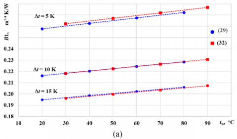
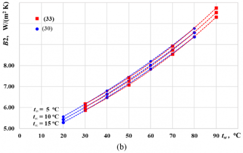
Figure 3. Values of B1 calculated from Eqns. (29) and (32) for Δt=5, 10 and 15 K as a function of the heating surface temperature varying in the range tw=20 – 90℃ (a) compared with values of B2 calculated from Eqns. (30) and (33) for t∞= 5, 10 and 15 K (Δt=tw – t∞) as a function of the heating surface temperature varying in the range tw=20 – 90℃ (b)
Figure 4. Comparison of values of B1·B2 calculated from Eqns. (34) (blue circles) and (35) (red squares). Eq. (36), shown in the box, is the result of the approximation of the curves obtained using Eq. (34)
3.1.3 Investigation of the influence of tw and Δt on the values of B1 and B2
Having determined t∞ and tav and the thermodynamic properties of air for given values of tw=90, 80, 70, 60, 50, 40, 30 and 20℃, together with Δt=5, 10, 15, 20, 40 and 60 K, the values of B1, B2 and their product were calculated. Some of the results of these simulation calculations, for Δt=5, 10 and 15 K, are summarized in Table 1 and Figure 3.
From the variability of B1 (29) and B2 (30) in the temperature range tw=0 – 90℃ for the set Δt=5, 10, 15, 20, 25 and 30 K, and the resulting values of t∞, tav, the following approximation relationships were determined:
B1=3.503.10-4 . Δt -0.2315. tw + 0.3914 . Δt -0.2661, (32)
$\begin{aligned} B 2= & \left(-2.457 \cdot 10^{-2} \Delta t+4.800\right) \cdot \\ & e^{\left(1.418 \cdot 10^{-5} \cdot \Delta t+9.168 \cdot 10^{-3}\right) \cdot t_w}\end{aligned}$, (33)
The calculated values of B1 from (29) and (32), and B2 from (30) and B2 (33) are compared graphically in Figure 3, in which, as in Table 1, the presentation is limited only to example values obtained for the range tw=20 – 90℃, and Δt=5, 10 and 15 K.
Apart from the values of B1 and B2, on the basis of which relationships (32) and (33) were derived, the values of their product B1·B2 were also calculated (see Table 1). To calculate them, the formulas obtained from the conversions of (29) and (30) as well as (32) and (33) to (34) and (35) were used:
$B 1 \cdot B 2=\frac{1}{\lambda \cdot\left(\frac{g \cdot \beta \cdot \Delta t}{v \cdot a}\right)^{\frac{1}{4}}} \cdot \frac{\sigma \cdot\left(T_w^4-T_{\infty}^4\right)}{\Delta t}$, (34)
$\begin{gathered}B 1 \cdot B 2=\left(3.503 \cdot 10^{-4} \cdot \Delta t^{-0.2315} \cdot t_w+\right. \left.+0.3914 \cdot \Delta t^{-0.2661}\right) \cdot(-2.457 \cdot \left.10^{-2} \Delta t+4.800\right)\cdot e^{\left(1.418 \cdot 10^{-5} \cdot \Delta t+9.168 \cdot 10^{-3}\right) \cdot t_w} \end{gathered}$ (35)
The values of B1·B2 calculated from these formulas are given in the relevant columns of Table 1 and in Figure 4. Note that Table 1 lists only results obtained for Δt=5, 10 and 15 K, whereas Figure 4 contains all the curves for B1·B2 (tw, Δt). The curves marked with blue lines and circles are a graphic representation of Eq. (34), those with red lines and squares represent Eq. (35).
As a result of the approximations of the B1·B2 (tw) curves shown in Figure 4, obtained on the basis of equation (34) (blue circles and lines) for Δt=5, 10, 15, 20, 25 and 30 K, one universal relationship was obtained:
$\begin{array}{r}B 1 \cdot B 2=\left(2.0461 \cdot \Delta t^{-0.3306}\right) \cdot e^{\left(1.008 \cdot 10^{-2} \cdot e^{1.426 \cdot 10^{-3} \,\, \cdot \Delta t}\right) \cdot t_w},\end{array}$ (36)
The results of the calculations for given tw and Δt obtained with the aid of this universal relationship are listed in the last column of Table 1. Like those resulting from the previous approximation (35), they exhibit a slight (only 0.37 and 0.38%) average discrepancy in relation to the results obtained using the original Eq. (34). This discrepancy concerns the entire scope of the calculations, only partially visualized in Table 1.
3.1.4 Analysis of the influence of tw and Δt on CR values
The dependence on the radiative constant in the Nusselt-Rayleigh criterion relationship CR can be obtained by substituting into (28) one of three equivalent formulas for B1·B2: (34), (35) or (36). In the case of substitution (36) one obtains:
$\begin{aligned} C_R= & B 1 \cdot B 2 \cdot l^{\frac{1}{4}} \cdot \varepsilon=\left(2.0461 \cdot \Delta t^{-0.3306}\right) . e^{\left(1.008 \cdot 10^{-2} \cdot e^{1.426 \cdot 10^{-3} \,\, \cdot \Delta t}\right) \cdot t_w} \cdot l^{1 / 4} \cdot \varepsilon\end{aligned}$, (37)
The linear influence of the surface emissivity factor ε on CR, being obvious and predictable (CR=0 for ε=0 and CR=CR,max for ε=1); hence, by assuming ε=1.0, it was omitted at this stage of the calculations. In contrast, analysis of the influence of the characteristic linear dimension l on CR cannot be omitted, because through B1 (31) it influences the value of the Rayleigh number, by means of which the intensity of convective heat exchange is described. While it is customary in convection that CC ≠ f(Ra)=const, it does not also have to apply to radiative heat transfer, for which it has been neither tested nor proven.
Table 2 shows the values of CR and Ra obtained from relationship (37) for given values of the surface temperature tw=100, 90, 80, 70, 60, 50, 40, 30, 25, 20 and 15℃, three values of the undisturbed area temperature t∞=10, 5 and 0℃, the constant value of the emissivity coefficient ε=1.0, and the following values of the characteristic linear dimension l=0.5, 0.25, 0.15, 0.10, 0.05 and 0.01 m. The values of Ra given in the Table 2 were calculated, as in Table 1, using relationships (14 - 27) as a function of tav, but in order to keep Table 2 readable, it does not include the calculated values of a, β and ν.
Table 2. Results of CR and Ra calculations for given values of tw, t∞ and l and the assumed constant value of ε=1
|
Temp. |
B1.B2 |
l=0.50 m |
l=0.25 m |
l=0.15 m |
l=0.10 m |
l=0.05 m |
l=0.01 m |
|||||||
|
tw |
t∞ |
(36) |
CR(37) |
Ra.10-10 |
CR(37) |
Ra.10-9 |
CR(37) |
Ra.10-8 |
CR(37) |
Ra.10-8 |
CR(37) |
Ra.10-7 |
CR(37) |
Ra.10-5 |
|
℃ |
℃ |
1/m1/4 |
– |
– |
– |
– |
– |
– |
– |
– |
– |
– |
– |
– |
|
100 |
0 |
1.4161 |
1.1908 |
2.7625 |
1.0013 |
3.4531 |
0.8813 |
7.4588 |
0.7963 |
2.2100 |
0.6696 |
2.7625 |
0.4478 |
2.2100 |
|
90 |
0 |
1.2873 |
1.0825 |
2.6291 |
0.9103 |
3.2863 |
0.8011 |
7.0984 |
0.7239 |
2.1032 |
0.6087 |
2.6291 |
0.4071 |
2.1032 |
|
80 |
0 |
1.1792 |
0.9916 |
2.4736 |
0.8338 |
3.0920 |
0.7338 |
6.6787 |
0.6631 |
1.9789 |
0.5576 |
2.4736 |
0.3729 |
1.9789 |
|
70 |
0 |
1.0894 |
0.9161 |
2.2933 |
0.7703 |
2.8666 |
0.6780 |
6.1919 |
0.6126 |
1.8346 |
0.5152 |
2.2933 |
0.3445 |
1.8346 |
|
60 |
0 |
1.0167 |
0.8550 |
2.0849 |
0.7189 |
2.6061 |
0.6327 |
5.6293 |
0.5718 |
1.6679 |
0.4808 |
2.0849 |
0.3215 |
1.6679 |
|
50 |
0 |
0.9609 |
0.8080 |
1.8448 |
0.6795 |
2.3060 |
0.5980 |
4.9810 |
0.5404 |
1.4758 |
0.4544 |
1.8448 |
0.3039 |
1.4758 |
|
40 |
0 |
0.9234 |
0.7765 |
1.5688 |
0.6529 |
1.9610 |
0.5747 |
4.2358 |
0.5193 |
1.2551 |
0.4366 |
1.5688 |
0.2920 |
1.2551 |
|
30 |
0 |
0.9093 |
0.7646 |
1.2522 |
0.6430 |
1.5652 |
0.5659 |
3.3809 |
0.5113 |
1.0017 |
0.4300 |
1.2522 |
0.2875 |
1.0017 |
|
25 |
0 |
0.9149 |
0.7694 |
1.0769 |
0.6470 |
1.3462 |
0.5694 |
2.9077 |
0.5145 |
0.8616 |
0.4327 |
1.0769 |
0.2893 |
0.8616 |
|
20 |
0 |
0.9338 |
0.7853 |
0.8895 |
0.6603 |
1.1118 |
0.5812 |
2.4015 |
0.5251 |
0.7116 |
0.4416 |
0.8895 |
0.2953 |
0.7116 |
|
15 |
0 |
0.9744 |
0.8194 |
0.6889 |
0.6890 |
0.8611 |
0.6064 |
1.8600 |
0.5479 |
0.5511 |
0.4608 |
0.6889 |
0.3081 |
0.5511 |
|
100 |
5 |
1.4285 |
1.2012 |
2.5530 |
1.0101 |
3.1913 |
0.8890 |
6.8932 |
0.8033 |
2.0424 |
0.6755 |
2.5530 |
0.4517 |
2.0424 |
|
90 |
5 |
1.3024 |
1.0952 |
2.4143 |
0.9209 |
3.0179 |
0.8105 |
6.5187 |
0.7324 |
1.9315 |
0.6159 |
2.4143 |
0.4118 |
1.9315 |
|
80 |
5 |
1.1969 |
1.0065 |
2.2537 |
0.8464 |
2.8172 |
0.7449 |
6.0851 |
0.6731 |
1.8030 |
0.5660 |
2.2537 |
0.3785 |
1.8030 |
|
70 |
5 |
1.1103 |
0.9337 |
2.0685 |
0.7851 |
2.5856 |
0.6910 |
5.5850 |
0.6244 |
1.6548 |
0.5250 |
2.0685 |
0.3511 |
1.6548 |
|
60 |
5 |
1.0416 |
0.8758 |
1.8555 |
0.7365 |
2.3193 |
0.6482 |
5.0098 |
0.5857 |
1.4844 |
0.4925 |
1.8555 |
0.3294 |
1.4844 |
|
50 |
5 |
0.9912 |
0.8335 |
1.6111 |
0.7009 |
2.0138 |
0.6168 |
4.3499 |
0.5574 |
1.2888 |
0.4687 |
1.6111 |
0.3134 |
1.2888 |
|
40 |
5 |
0.9622 |
0.8091 |
1.3312 |
0.6804 |
1.6640 |
0.5988 |
3.5943 |
0.5411 |
1.0650 |
0.4550 |
1.3312 |
0.3043 |
1.0650 |
|
30 |
5 |
0.9637 |
0.8103 |
1.0114 |
0.6814 |
1.2642 |
0.5997 |
2.7307 |
0.5419 |
0.8091 |
0.4557 |
1.0114 |
0.3047 |
0.8091 |
|
25 |
5 |
0.9832 |
0.8268 |
0.8348 |
0.6952 |
1.0435 |
0.6119 |
2.2539 |
0.5529 |
0.6678 |
0.4649 |
0.8348 |
0.3109 |
0.6678 |
|
20 |
5 |
1.0255 |
0.8623 |
0.6462 |
0.7251 |
0.8077 |
0.6382 |
1.7446 |
0.5767 |
0.5169 |
0.4849 |
0.6462 |
0.3243 |
0.5169 |
|
15 |
5 |
1.1129 |
0.9359 |
0.4447 |
0.7870 |
0.5559 |
0.6926 |
1.2008 |
0.6259 |
0.3558 |
0.5263 |
0.4447 |
0.3519 |
0.3558 |
|
100 |
10 |
1.4425 |
1.2130 |
2.3535 |
1.0200 |
2.9418 |
0.8977 |
6.3543 |
0.8112 |
1.8828 |
0.6821 |
2.3535 |
0.4562 |
1.8828 |
|
90 |
10 |
1.3192 |
1.1093 |
2.2100 |
0.9328 |
2.7625 |
0.8210 |
5.9670 |
0.7418 |
1.7680 |
0.6238 |
2.2100 |
0.4172 |
1.7680 |
|
80 |
10 |
1.2168 |
1.0232 |
2.0448 |
0.8604 |
2.5560 |
0.7573 |
5.5210 |
0.6843 |
1.6359 |
0.5754 |
2.0448 |
0.3848 |
1.6359 |
|
70 |
10 |
1.1339 |
0.9535 |
1.8552 |
0.8018 |
2.3190 |
0.7056 |
5.0090 |
0.6376 |
1.4842 |
0.5362 |
1.8552 |
0.3586 |
1.4842 |
|
60 |
10 |
1.0699 |
0.8997 |
1.6381 |
0.7566 |
2.0476 |
0.6659 |
4.4228 |
0.6017 |
1.3104 |
0.5059 |
1.6381 |
0.3383 |
1.3104 |
|
50 |
10 |
1.0266 |
0.8633 |
1.3899 |
0.7259 |
1.7374 |
0.6389 |
3.7528 |
0.5773 |
1.1120 |
0.4855 |
1.3899 |
0.3246 |
1.1120 |
|
40 |
10 |
1.0094 |
0.8488 |
1.1069 |
0.7138 |
1.3836 |
0.6282 |
2.9886 |
0.5677 |
0.8855 |
0.4773 |
1.1069 |
0.3192 |
0.8855 |
|
30 |
10 |
1.0351 |
0.8704 |
0.7844 |
0.7320 |
0.9805 |
0.6442 |
2.1179 |
0.5821 |
0.6275 |
0.4895 |
0.7844 |
0.3273 |
0.6275 |
|
25 |
10 |
1.0793 |
0.9076 |
0.6068 |
0.7632 |
0.7585 |
0.6717 |
1.6384 |
0.6069 |
0.4855 |
0.5104 |
0.6068 |
0.3413 |
0.4855 |
|
20 |
10 |
1.1709 |
0.9846 |
0.4174 |
0.8280 |
0.5217 |
0.7287 |
1.1270 |
0.6584 |
0.3339 |
0.5537 |
0.4174 |
0.3703 |
0.3339 |
|
15 |
10 |
1.3981 |
1.1756 |
0.2154 |
0.9886 |
0.2692 |
0.8701 |
0.5815 |
0.7862 |
0.1723 |
0.6611 |
0.2154 |
0.4421 |
0.1723 |
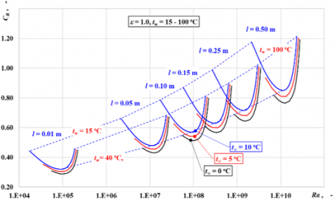
Figure 5. Graphical interpretation of the influence of tw, t∞, and l on CR expressed by the function CR=f(Δt) assuming ε=1 in relationship (37)
Figure 6. The influence of tw, t∞, and l on CR, calculated from the dependence (37) assuming ε =1, expressed in the form of the function CR=f(Ra)
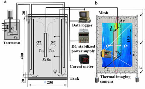
Figure 7. Diagram of the experimental apparatus for examining: a) free convective heat transfer in water, using the balance method and an isothermal vertical plate, b) total convective and radiative heat transfer in air, obtained by the use of balance method, and the convective only, obtained by the gradient method, with the additional use of IR camera with detection mesh [71]
From among the various possible graphical presentations of the results in Table 2, it was decided to show the relationships CR=f(Δt) in Figure 5 and CR=f(Ra) in Figure 6. In both figures the results for the same temperature of the undisturbed area are indicated for t∞=10℃ by a blue line, for t∞=5℃ by a red one, and for t∞=0℃ by a black one. In Figure 5, the beginnings of the curves related to the heated surface temperature tw=15℃ are on the left side of the graph, those for tw=100℃ on the right. Because these positions are correlated with the values of Δt, they are easier to analyse. In the case of Figure 6, where there is no such correlation, the two outermost dashed blue lines connecting the points with the highest and lowest surface temperatures tw=15 and 100℃ and a third line of minimum CR values for tw ≈ 40℃ have been added, but only for t∞=10℃ these lines were created on the basis of the data shown in bold in Table 2.
Figures 5 and 6 show that the function CR in radiative heat exchange is not constant, as was the case with CC, which was correct for convective heat exchange. The function CR defined in this way depends on the coefficient CR of the emissivity ε, the temperature conditions tw and t∞, the area of the heated surface l, which determine the Rayleigh number, but also on the thermodynamic properties of air a, β and ν, which are included in Ra.
3.1.5 Final solution in the form of CC+R and its application
Knowing the convective constant CC and the radiative function CR, described by Eq. (37), one can determine the value of CC+R=CC+CR from Eq. (28) depending on the criterion dependence (12), which in turn opens up the possibility of determining the total (convective-radiative) heat flux QC+R from any vertical surface:
$C_{C+R}=C_C+B 1 \cdot B 2 \cdot l^{\frac{1}{4}} \cdot \varepsilon=\frac{N u_{C+R}}{R a^{\frac{1}{4}}}=\frac{\alpha_{C+R} \quad \cdot l}{\lambda \cdot R a^{1 / 4}} \quad$, (38)
$Q_{C+R}=\frac{\lambda \cdot A}{l} \cdot \Delta t \cdot R a^{1 / 4} \cdot\left(C_C+B 1 \cdot B 2 \cdot l^{\frac{1}{4}} \cdot \varepsilon\right)$. (39)
At first glance, these equations seem complicated and require more time to obtain the results than existing solutions. However, their advantage is that, after measuring tw, t∞ and ε, one can use a thermal imaging camera with appropriate software to directly determine the heat flux from any heated surface of known dimensions l, e.g., a building surface. For this purpose, Eqns. (20), (24)-(27), (31), (37), (39) should only include Δt, tav, ε and l, along with the literature value of the constant of free convection from a vertical plate, e.g., CC=0.569 [71]. In the case of horizontal surfaces, this constant and the exponent n will have different values depending on criterion (2) and hence, the entire solution.
In this solution, the heat exchange is assumed by default to be in the laminar range, i.e. from Racr,I ≈ 103 to Racr,II ≈ 109 (Racr,air=2.0.108 and Racr,water=3.4.109 [79] for uniform flux) because above and below this range, heat transfer takes place by conduction or transition convection; for the latter, there are other values of the constants in Nusselt-Rayleigh criterion dependence (6) and (20), e.g. CC=0.135 and n=1/3.
4.1 Experimental validation of the solution
At the very beginning of this section, it should be noted that the titular validation concerns only the correctness of the solution for the constant CC+R depending on Nu=CC+R.Ra1/4, describing convective-radiative heat transfer. The tests of convective heat transfer in water obtained by the use of the balance method (a) and convective heat transfer in air obtained by the gradient method with the use of thermal imaging camera with a detection mesh, as well as combined convective and radiative heat transfer in air obtained by the use of balance method without a camera and mesh (b) were carried out on the test stand shown diagrammatically in Figure 7. Since the details of these studies have already been described in the study [71], they have been omitted here, except for the results. Based on an analysis of the relationships between the measured values of CC, B1.B2 and CC+, these results were used to develop an empirical relationship (39) and to verify it experimentally. On the test stand shown in Figure 7a, the balance method was used to determine the value of CC,water=0.536 for an isothermal vertical plate and free convection in water, while on the test stand illustrated in Figure 6b, the new gradient method of detecting convection with a thermal imaging camera equipped with a detecting mesh was used to determine the value of CC,air=0.579 for air [71]. On the same test stand, but using the balance method, the constant value of CC+R=1.220 was obtained for air, which covers both convection and radiation heat transfer [71].
4.1.1 Research test stand
The main element of the above test stands was a thin double-sided and symmetrically heated vertical plate of height h=0.15 m, width b=0.075 m and thickness s=0.003 m. The plate was made from three layers of copper-laminated glass-epoxy composite, each 0.6 mm thick. The outer layers (LAM100X160E0.6), laminated on one side with a copper layer of thickness g=35 mm, consisted of two surface resistance thermometers with resistances 235.1 W and 240.7 W, located on both sides of the plate. The middle layer (LAM100X160ED0.6), laminated on both sides with 18 mm thick copper layers, was a two-sided heating resistance heater with 44.8 W and 45.2 W resistances, which was powered by two power supplies with power N=30 W, voltage U=0 - 10 V and current I=0 - 3 A.
Both thermometers and heaters were made by etching the resistance paths in copper by photolithography. More information, including dimensions, drawings and photos, on the production and calibration of the heater used in these tests can be found in the study [71]. A similar concept of a double-sided isothermal plate set obliquely was used in the study [80].
4.1.2 The study of radiative-convective heat transfer in air
The convective-radiative heat transfer study was carried out in the traditional way, by gradually increasing the heating power of the heaters. Since the heat exchange was symmetrical, as evidenced by practically the same surface temperatures on both sides of the plate, the heater was connected in series. After establishing the thermodynamic equilibrium tw, tav and Δt, the result was recorded, the power increased and another measurement started.
The results of the voltage and direct current variation of the heater Ii, A, Ui, V, obtained in tabular form, enabled the heat flux Qi transferred to the air from the Ni power to be calculated. It was decided not to take into account the heat loss flux at the edges owing to the small surface area (thickness s=3 mm).
Then, based on the values of λi=f(tav) obtained from (27) and the dimension b=0.075 m of the plate, Nui was calculated from Eq. (11).
In turn, knowing the temperatures of both sides of the plate surface twI,i and twII,i and the air in the undisturbed area t∞,i, the average temperatures of the plate surface and air tw,i, tav,i and Δti could be calculated, from which the physical properties of the air could be determined from (24), (25) and (26) and consequently, the Rayleigh numbers for h=0.15 m and Δti from Eq. (31).
The last procedure for processing the experimental data was to calculate the individual values of CC+R=NuC+R/Ra1/4, some of which (diamonds in Figure 6) along with the mean are given in the experimental part of Table 3. The last row of Table 3 shows the averages of the results of all the research, both experimental and theoretical.
Paper [71] gives identical results, obtained on the same stand for air, but the content of Table 3 has changed. This shows the results of convective transfer, not tabulated in the study [71], and thus the differences in averaging the tabular data. On the other hand, the difference in averaging all the results CC+R,av=1.197 (maximum relative uncertainty δCexp.= 8.5%) differs slightly from that given in the study [71]. CC+R,av=1.220 results from the use of other formulas to determine the physical properties of air in both papers. The present Eqns. (24) - (27) are correlated with tav and the previous ones with other constants from Tav.
In the study [71], apart from the convective-radiative heat transfer in air, tests of free convection in water, in which radiative heat transfer can be omitted, were carried out on a different stand (see Figure 7a), but with the same heating plate. The criterion dependence obtained in those studies for water takes the following form:
NuC=(0.536 ± 0.073) . Ra 0.25 (Ra =2.106 – 8.108), (40)
This dependence is 5.8% less than (20), but because it was obtained as a result of experimental studies carried out in a similar way and on the same heating plate, we decided to use it to validate the correctness of the solution. Detailed calculations of this validation can be found in the study [78]. The maximum relative uncertainty δCexp.=±13.7% (for the experiment conducted in water) has been included in Eq. (40).
Table 3 also lists the results obtained from processing the experimental data using equations derived from theoretical considerations. The values of function B1·B2, given in the theoretical part of Table 3, were based on Eq. (36), in which the experimental values of tw and Δt were substituted.
Table 3. Results of overall (convective and radiative) heat transfer tests from a vertical plate in air
|
Heating power N |
Temperature |
Experimental results |
Comparison with theory |
|||||||||
|
NuC+R |
Ra .10-6 |
CC+R |
B1.B2 |
CR |
CC+R |
CR |
CC+R |
|||||
|
ε=0.884 |
ε=0.932 |
|||||||||||
|
tw |
t∞ |
tav |
∆t |
(11) |
(31) |
(13) |
(36) |
(37) |
(41) |
(37) |
(41) |
|
|
W |
℃ |
℃ |
℃ |
K |
- |
- |
- |
m-1/4 |
- |
- |
- |
- |
|
Series I |
||||||||||||
|
1.0 |
28.5 |
23.9 |
26.2 |
4.6 |
53.207 |
1.496 |
1.521 |
1.642 |
0.903 |
1.439 |
0.952 |
1.488 |
|
1.8 |
32.8 |
24.1 |
28.4 |
8.7 |
53.372 |
2.700 |
1.317 |
1.396 |
0.768 |
1.304 |
0.810 |
1.346 |
|
2.9 |
37.4 |
24.4 |
30.9 |
13.0 |
55.759 |
3.900 |
1.255 |
1.283 |
0.706 |
1.242 |
0.744 |
1.280 |
|
4.0 |
42.3 |
24.9 |
33.6 |
17.4 |
57.362 |
5.009 |
1.213 |
1.228 |
0.676 |
1.212 |
0.713 |
1.249 |
|
5.1 |
46.7 |
24.9 |
35.8 |
21.8 |
57.946 |
6.071 |
1.167 |
1.197 |
0.658 |
1.194 |
0.694 |
1.230 |
|
5.9 |
50.7 |
25.1 |
37.9 |
25.6 |
56.940 |
6.920 |
1.110 |
1.186 |
0.652 |
1.188 |
0.688 |
1.224 |
|
6.9 |
54.4 |
25.2 |
39.8 |
29.2 |
58.694 |
7.672 |
1.115 |
1.183 |
0.651 |
1.187 |
0.686 |
1.222 |
|
7.8 |
57.7 |
25.3 |
41.5 |
32.4 |
59.313 |
8.321 |
1.104 |
1.186 |
0.653 |
1.189 |
0.688 |
1.224 |
|
9.1 |
61.8 |
25.3 |
43.6 |
36.5 |
60.959 |
9.095 |
1.110 |
1.195 |
0.658 |
1.194 |
0.693 |
1.229 |
|
Series II |
||||||||||||
|
5.0 |
48.5 |
25.9 |
37.2 |
22.6 |
54.304 |
6.181 |
1.089 |
1.205 |
0.663 |
1.199 |
0.699 |
1.235 |
|
6.1 |
52.2 |
25.8 |
39.0 |
26.4 |
57.191 |
7.015 |
1.111 |
1.193 |
0.656 |
1.192 |
0.692 |
1.228 |
|
6.9 |
55.3 |
25.6 |
40.5 |
29.7 |
57.480 |
7.743 |
1.090 |
1.188 |
0.654 |
1.190 |
0.689 |
1.225 |
|
8.4 |
59.2 |
25.7 |
42.5 |
33.5 |
61.357 |
8.488 |
1.137 |
1.193 |
0.656 |
1.192 |
0.692 |
1.228 |
|
9.2 |
63.1 |
25.4 |
44.3 |
37.7 |
59.276 |
9.303 |
1.073 |
1.200 |
0.660 |
1.196 |
0.696 |
1.232 |
|
10.1 |
66.1 |
25.2 |
45.7 |
40.9 |
60.120 |
9.895 |
1.072 |
1.210 |
0.666 |
1.202 |
0.702 |
1.238 |
|
Average for the 15 results listed in this table |
1.166 |
1.246 |
0.685 |
1.221 |
0.723 |
1.259 |
||||||
|
Average value for all 27 results shown in Figure 6 |
1.197 |
1.239 |
0.682 |
1.218 |
0.719 |
1.255 |
||||||
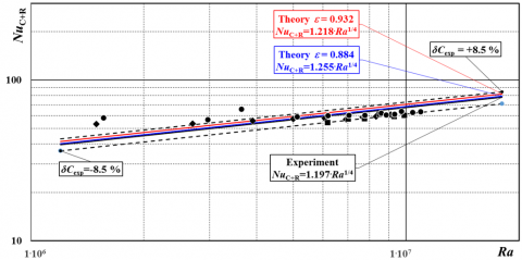
Figure 8. The results of the experimental tests, some of which - from Series I (diamonds) and Series II (squares) - are included in Table 3, and the remaining (Series III) experimental points (shown by dots) are not shown in Table 3. The black line shows the approximation of all the experimental results (41). The theoretical solution obtained for ε=0.884 is shown by the blue line, and the one for ε=0.932 by the red line
Further, from Eq. (37), the constant CR was calculated for the two given for experimental plate emissivities ε=0.884 (estimated experimentally) and ε=0.932 (calculated from experimental data) [71] of a plate with a characteristic linear dimension of l=0.15 m. Without enquiring which of these emissivities is closer to reality, both values CR and CC+R were calculated.
The constant CC+R is the sum of the convection constant CC (40) and the radiation constant CR:
$C_{C+R}=C_C+C_R$. (41)
The results of these calculations were also subjected to double averaging with reference to the sample data listed in Table 3 and to all the results shown in Figure 8. The maximum relative uncertainty for the experiment in air (δCexp.=±8.5%) has been adopted here.
At the end of the experimental research and theoretical considerations, it had to be checked whether the results fell within the laminar for air range Ra < Racr,sir=2.108 [79]. First, the experimental relationship (40) was checked: since this was obtained for water with the maximum number of Ramax ≈ 8.108 < Racr,water=3.4.109 [79], it also raised no objections.
The results of the experimental studies published in the study [71] were used to validate the solution. Therefore, they cannot be suspected of being biased, even to a minimal degree. It is even more difficult to imagine the possibility of matching the results of theoretical considerations with experimental data. In this situation, the discrepancy between the experimental and theoretical values of CC+R,av – 1.75% (for ε=0.884) and 4.85% (for ε=0.932) – offers incontrovertible evidence confirming both the reliability of the experiment and the correctness of the solution of the empirical Eq. (39) with coefficient (36).
Having ensured that the solutions are correct, one can begin to outline its possible practical applications, which may be:
- a simple way of determining the heat loss from any external wall, building envelope, façade of a building, etc., or the heat flux transferred from internal walls inside a building, based on knowledge of: the value of its area A, characteristic linear dimension l (height), temperature tw, the surrounding temperature t∞ and the approximate (e.g., tabular) value the surface emissivity ε, which has little effect on the result (ΔQ ≈ 3% for Δε=0.05%).
- if the building surfaces under consideration are not vertical, isothermal or if Ra > Racr (CC (20) or (40)), then it suffices to substitute the relevant values of CC in Eq. (39).
- the development of dedicated software for a thermal imaging camera, which is based on the temperature of the heated surface tw and the air in surrounding t∞, which are in thermodynamic equilibrium with the surroundings, and the emissivities of the surface and the surroundings. With such a programme, a properly modified camera, in addition to its current applications in energy audits of buildings [62, 81-85], or recently for measuring air velocity [21], net heat flux [86] or heat flux and hot spot temperature in machining process [87], with the use of infrared image sequences, could also measure the total (convection-radiative) energy flux emitted from walls.
This work was supported by the Icelandic Research Fund (Grant No. 184949); the Swedish Research Council (Grant No. 2020-05110).
|
a |
coefficient of thermal diffusivity, m2/s |
|
A |
surface area, m2 |
|
b |
width of the plate, m |
|
B1 |
function, K.m7/4/W (29), (32) |
|
B2 |
function, W/(m2.K) (30), (33) |
|
cp |
specific heat, J/(kg·K) |
|
C |
coefficient in the Rayleigh–Nusselt equation |
|
g |
acceleration due to gravity, m/s2 |
|
h |
height of the plate, m |
|
I |
current, A |
|
l |
characteristic length, m |
|
n |
exponent |
|
N |
heater power, W |
|
Nu |
Nusselt number, dimensionless |
|
Ra |
Rayleigh number, dimensionless |
|
t,T |
temperature, ℃, K |
|
q |
flux density, W/m2 |
|
Q |
heat flux, W |
|
U |
voltage, V |
|
Greek symbols |
|
|
α |
heat-transfer coefficient, W/(m2·K) |
|
β |
coefficient of thermal expansion, 1/K |
|
$\delta$ |
uncertainty |
|
ε |
surface emissivity |
|
σ |
Stefan-Boltzmann constant, W/(m2·K4) |
|
Δ |
difference |
|
λ |
thermal conductivity, W/(m·K) |
|
$\mu$ |
dynamic viscosity, kg/(m·s) |
|
ρ |
density, kg/m3 |
|
ν |
kinematic viscosity, m2/s |
|
Subscripts |
|
|
av |
average |
|
cr |
critical |
|
C |
convective |
|
in |
inlet |
|
max |
maximum |
|
loss |
losses |
|
out |
outlet |
|
R |
radiative |
|
w |
wall |
|
∞ |
in surroundings |
[1] Raznjevic, K. (1995). Handbook of Thermodynamic Tables. Begell House. New York.
[2] Handbook: Fundamentals - IP Edition. Atlanta: American Society of Heating, Refrigerating and Air-Conditioning Engineers. 2009. https://www.academia.edu/10884294/ASHRAE_handbook_fundamental, accessed on 15 March 2023.
[3] Modest, M.F. (2013). Radiative Heat Transfer. 3th Edition, McGraw-Hill, New York.
[4] Howell, J.R. Mengüc, M.P., Daun, K., Siegel R. (2021). Thermal Radiation Heat Transfer, 7th Edition, CRC Press.
[5] Ficker, T. (2019). General model of radiative and convective heat transfer in buildings: Part II: Convective and radiative heat losses. Acta Polytechnica, 59(3): 224-237. https://doi.org/10.14311/AP.2019.59.0224
[6] Karatas, H., Derbentli, T. (2018). Natural convection and radiation in rectangular cavities with one active vertical wall. International Journal of Thermal Sciences, 123: 129-139. https://doi.org/10.1016/j.ijthermalsci.2017.09.006
[7] Pudlik, W. (2012). Wymiana i Wymienniki Ciepła (Heat Transfer and Heat Exchangers) Gdańsk University of Tech. Publishing House, Gdańsk 2012, p. 232. https://pbc.gda.pl/Content/4404/wymiana-i-wymienniki-final.pdf.
[8] Stasiek, J. (1985). Application of the generalized configuration factors and the principle of surface transformation to radiant heat exchange in systems with optically active medium. Mechanika, 49: 386.
[9] Ozisik, M.N. (1987). Interaction of Radiation with Convection in Handbook of Single-phase Convective Heat Transfer. John Wiley & Sons, New York.
[10] Lewandowski, W.M., Khubeiz, J.M., Kubski, P., Bieszk, H., Wilczewski, T., Szymański, S. (1998). Natural convection heat transfer from complex surface. International Journal of Heat and Mass Transfer, 41(12): 1857-1868. https://doi.org/10.1016/s0017-9310(97)00240-8
[11] Misale, M., Fossa, M., Tanda, G. (2014). Investigation of free convection in a vertical water channel. Experimental Thermal and Fluid Science, 59: 252-257. https://doi.org/10.1016/j.expthermflusci.2014.01.022
[12] Lewandowski, W.M., Radziemska, E., Buzuk, M., Bieszk, H. (2000). Free convection heat transfer and fluid flow above horizontal rectangular plates. Applied Energy, 66(2): 177-197. https://doi.org/10.1016/S0306-2619(99)00024-0
[13] Lewandowski, W.M., Kubski, P., Bieszk, H. (1994). Heat transfer from polygonal horizontal isothermal surfaces. International Journal of Heat and Mass Transfer, 37(5): 855-864. https://doi.org/10.1016/0017-9310(94)90121-X
[14] Lewandowski, W.M., Bieszk, H., Cieslinski, J. (1992). Free convection from horizontal screened plates. Waerme-und Stoffuebertragung; (Germany), 27(8): 481-488. https://doi.org/10.1007/BF01590049
[15] Cieśliński, J., Pudlik, W. (1988). Laminar free-convection from spherical segments. International Journal of Heat and Fluid Flow, 9(4): 405-409. https://doi.org/10.1016/0142-727X(88)90007-0
[16] Lewandowski, W.M., Kubski, P., Khubeiz, J.M. (1993). Laminar free convection heat transfer from a horizontal ring. Wärme-und Stoffübertragung, 29(1): 9-16. https://doi.org/10.1007/BF01577454
[17] Cieśliński, J.T., Smolen, S., Sawicka, D. (2021). Free convection heat transfer from horizontal cylinders. Energies, 14(3): 559. https://doi.org/10.3390/en14030559
[18] Lewandowski, W.M., Kubski, P., Khubeiz, J.M. (1992). Natural convection heat transfer from round horizontal plate. Waerme-und Stoffuebertragung; (Germany), 27(5): 281-287. https://doi.org/10.1007/BF01589965
[19] Lewandowski, W.M., Ryms, M., Denda, H., Klugmann-Radziemska, E. (2014). Possibility of thermal imaging use in studies of natural convection heat transfer on the example of an isothermal vertical plate. International Journal of Heat and Mass Transfer, 78: 1232-1242. https://doi.org/10.1016/j.ijheatmasstransfer.2014.07.024
[20] Schaub, M., Kriegel, M., Brandt, S. (2019). Experimental investigation of heat transfer by unsteady natural convection at a vertical flat plate. International Journal of Heat and Mass Transfer, 136: 1186-1198. https://doi.org/10.1016/j.ijheatmasstransfer.2019.03.089
[21] Ryms, M., Tesch, K., Lewandowski, W.M. (2021). The use of thermal imaging camera to estimate velocity profiles based on temperature distribution in a free convection boundary layer. International Journal of Heat and Mass Transfer, 165: 120686. https://doi.org/10.1016/j.ijheatmasstransfer.2020.120686
[22] Lei, C., Patterson, J.C. (2003). A direct three-dimensional simulation of radiation-induced natural convection in a shallow wedge. International Journal of Heat and Mass Transfer, 46(7): 1183-1197. https://doi.org/10.1016/S0017-9310(02)00401-5
[23] Liu, X., Gong, G., Cheng, H. (2014). Combined natural convection and radiation heat transfer of various absorbing-emitting-scattering media in a square cavity. Advances in Mechanical Engineering, 6: 403690. https://doi.org/10.1155/2014/403690
[24] Zhou, L., Liu, J., Huang, Q., Wang, Y. (2019). Analysis of combined natural convection and radiation heat transfer in a partitioned rectangular enclosure with semitransparent walls. Transactions of Tianjin University, 25: 472-487. https://doi.org/10.1007/s12209-019-00208-9
[25] Wang, Y., Yang, J., Zhang, X., Pan, Y. (2015). Effect of surface thermal radiation on natural convection and heat transfer in a cavity containing a horizontal porous layer. Procedia Engineering, 121: 1193-1199. https://doi.org/10.1016/j.proeng.2015.09.137
[26] Cabanillas, R.E., Estrada, C.A., Alvarez, G. (2002). Combined natural convection and radiation heat transfer in an open tilted cavity. WIT Transactions on Engineering Sciences, 35. https://doi.org/10.2495/HT020101
[27] Wang, Z., Yang, M., Li, L., Zhang, Y. (2011). Combined heat transfer by natural convection–conduction and surface radiation in an open cavity under constant heat flux heating. Numerical Heat Transfer, Part A: Applications, 60(4): 289-304. https://doi.org/10.1080/10407782.2011.594415
[28] Lugarini, A., Franco, A.T., Junqueira, S.L., Lage, J.L. (2018). Natural convection and surface radiation in a heated wall, C-shaped fracture. ASME Journal of Heat and Mass Transfer, 140(8): 082501. https://doi.org/10.1115/1.4039643
[29] Lacona, E., Taine, J. (2001). Holographic interferometry applied to coupled free convection and radiative transfer in a cavity containing a vertical plate between 290 and 650 K. International Journal of Heat and Mass Transfer, 44(19): 3755-3764. https://doi.org/10.1016/S0017-9310(01)00027-8
[30] Qasem, N.A.A., Imteyaz, B., Ben-Mansour, R., Habib, M.A. (2017). Effect of radiation heat transfer on naturally driven flow through parallel-plate vertical channel. Arabian Journal for Science and Engineering, 42: 1817-1829. https://doi.org/10.1007/s13369-016-2319-8
[31] Lewandowski, W.M., Ryms, M., Denda, H. (2017). Infrared techniques for natural convection investigations in channels between two vertical, parallel, isothermal and symmetrically heated plates. International Journal of Heat and Mass Transfer, 114: 958-969. https://doi.org/10.1016/j.ijheatmasstransfer.2017.06.120
[32] Lewandowski, W.M., Ryms, M., Denda, H. (2018). Natural convection in symmetrically heated vertical channels. International Journal of Thermal Sciences, 134: 530-540. https://doi.org/10.1016/j.ijthermalsci.2018.08.036
[33] Krishna Sabareesh, R., Prasanna, S., Venkateshan, S.P. (2010). Investigations on multimode heat transfer from a heated vertical plate. Journal of Heat Transfer, 132(3): 032501. https://doi.org/10.1115/1.4000055
[34] Shati, A.K.A., Blakey, S.G., Beck, S.B.M. (2012). A dimensionless solution to radiation and turbulent natural convection in square and rectangular enclosures. Journal of Engineering Science and Technology, 7(2): 257-279.
[35] Pantokratoras, A. (2014). Natural convection along a vertical isothermal plate with linear and non-linear Rosseland thermal radiation. International Journal of Thermal Sciences, 84: 151-157. https://doi.org/10.1016/j.ijthermalsci.2014.05.015
[36] Cheesewright, R. (1968). Turbulent natural convection from a vertical plane surface. ASME Journal of Heat and Mass Transfer, 90(1): 1-6. https://doi.org/10.1115/1.3597453
[37] Hasan, M.M., Eichhorn, R. (1979). Local nonsimilarity solution of free convection flow and heat transfer from an inclined isothermal plate. ASME Journal of Heat and Mass Transfer, 101(4): 642-647. https://doi.org/10.1115/1.3451050
[38] Fujii, T., Imura, H. (1972). Natural-convection heat transfer from a plate with arbitrary inclination. International Journal of Heat and Mass Transfer, 15(4): 755-767. https://doi.org/10.1016/0017-9310(72)90118-4
[39] Hossain, M.A., Takhar, H.S. (1996). Radiation effect on mixed convection along a vertical plate with uniform surface temperature. Heat and Mass Transfer, 31(4): 243-248. https://doi.org/10.1007/BF02328616
[40] Cao, K., Baker, J. (2015). Non-continuum effects on natural convection–radiation boundary layer flow from a heated vertical plate. International Journal of Heat and Mass Transfer, 90: 26-33. https://doi.org/10.1016/j.ijheatmasstransfer.2015.05.014
[41] Arpaci, V.S. (1968). Effect of thermal radiation on the laminar free convection from a heated vertical plate. International Journal of Heat and Mass Transfer, 11(5): 871-881. https://doi.org/10.1016/0017-9310(68)90130-0
[42] Reddy, M.G. (2014). Influence of thermal radiation, viscous dissipation and hall current on MHD convection flow over a stretched vertical flat plate. Ain Shams Engineering Journal, 5(1): 169-175. https://doi.org/10.1016/j.asej.2013.08.003
[43] Venugopal, G., Deiveegan, M., Balaji, C., Venkateshan, S.P. (2008). Simultaneous retrieval of total hemispherical emissivity and specific heat from transient multimode heat transfer experiments. Journal of Heat Transfer, 130(6): 061601. https://doi.org/10.1115/1.2891221
[44] Venugopal, G., Balaji, C., Venkateshan, S.P. (2008). A correlation for laminar mixed convection from vertical plates using transient experiments. Heat and Mass Transfer, 44(12): 1417-1425. https://doi.org/10.1007/s00231-008-0380-x
[45] Bhowmik, H., Faisal, A. (2017). Experimental analyses of natural convection and radiation heat transfer from a horizontal cylinder. 10th International Conference on Thermal Engineering: Theory and Applications, February 26-28, 2017, Muscat, Oman, pp. 1-5.
[46] Popiel, C.O., Wojtkowiak, J., Bober, K. (2007). Laminar free convective heat transfer from isothermal vertical slender cylinder. Experimental Thermal and Fluid Science, 32(2): 607-613. https://doi.org/10.1016/j.expthermflusci.2007.07.003
[47] Kobus, C.J., Wedekind, G.L. (1995). An experimental investigation into forced, natural and combined forced and natural convective heat transfer from stationary isothermal circular disks. International Journal of Heat and Mass Transfer, 38(18): 3329-3339. https://doi.org/10.1016/0017-9310(95)00096-R
[48] Ali, M. (2009). Natural convection heat transfer along vertical rectangular ducts. Heat and Mass Transfer, 46: 255-266. https://doi.org/10.1007/s00231-009-0561-2
[49] Zeyghami, M., Rahman, M.M. (2015). Analysis of combined natural convection and radiation heat transfer using a similarity solution. Energy Research Journal, 6(2): 64-73. https://doi.org/10.3844/erjsp.2015.64.73
[50] Jannot, M., Kunc, T. (1998). Onset of transition to turbulence in natural convection with gas along a vertical isotherm plane. International Journal of Heat and Mass Transfer, 41(24): 4327-4340. https://doi.org/10.1016/S0017-9310(98)00068-4
[51] Clausing, A.M., Berton, J.J. (1989). An experimental investigation of natural convection from an isothermal horizontal plate. ASME Journal of Heat and Mass Transfer, 111(4): 904-908. https://doi.org/10.1115/1.3250804
[52] Eckert, E.R.G., Jackson, T.W. (1950). Analysis of turbulent free-convection boundary layer on flat plate (No. NACA-TN-2207).
[53] Hossain, M.A., Rees, D.A.S., Pop, I. (1998). Free convection-radiation interaction from an isothermal plate inclined at a small angle to the horizontal. Acta Mechanica, 127(1-4): 63-73. https://doi.org/10.1007/BF01170363
[54] Cess, R.D. (1966). The interaction of thermal radiation with free convection heat transfer. International Journal of Heat and Mass Transfer, 9(11): 1269-1277. https://doi.org/10.1016/0017-9310(66)90119-0
[55] England, W.G., Emery, A.F. (1969). Thermal radiation effects on the laminar free convection boundary layer of an absorbing gas. ASME Journal of Heat and Mass Transfer, 91(1): 37-44. https://doi.org/10.1115/1.3580116
[56] Ramesh, N., Balaji, C., Venkateshan, S.P. (2000). Effect of radiation on natural convection in an L-shaped corner. Experiments in Fluids, 28(5): 448-454. https://doi.org/10.1007/s003480050404
[57] Kimura, K. (2016). Scientific Basis of Air Conditioning. Edition: Second Edition 2016 Publisher: International Research Institute on Human Environment ISBN: 978-4-9907042-3-0.
[58] Lewandowski, W.M., Lewandowska-Iwaniak, W. (2014). The external walls of a passive building: A classification and description of their thermal and optical properties. Energy and Buildings, 69: 93-102. https://doi.org/10.1016/j.enbuild.2013.10.021
[59] Sobota, T., Taler, J. (2018). Determination of heat losses through building partitions. In MATEC Web of Conferences, 240: 05030. https://doi.org/10.1051/matecconf/201824005030
[60] Ficker, T. (2019). General model of radiative and convective heat transfer in buildings: Part I: Algebraic model of radiative heat transfer. Acta Polytechnica, 59(3): 211-223. https://doi.org/10.14311/AP.2019.59.0211
[61] Kulacki, F.A., Nagle, M.E., Cassen, P. (1974). Studies of heat source driven natural convection (No. NASA-TM-X-70232). Technical Report 3746-2, Grant NGR 36-008-205.
[62] Ohlsson, K.E.A., Olofsson, T. (2014). Quantitative infrared thermography imaging of the density of heat flow rate through a building element surface. Applied Energy, 134: 499-505. https://doi.org/10.1016/j.apenergy.2014.08.058
[63] Wernik, J. (2017). Investigation of heat loss from the finned housing of the electric motor of a vacuum pump. Applied Sciences, 7(12): 1214. https://doi.org/10.3390/app7121214
[64] Sakin, M., Kaymak-Ertekin, F., Ilicali, C. (2009). Convection and radiation combined surface heat transfer coefficient in baking ovens. Journal of Food Engineering, 94(3-4): 344-349. https://doi.org/10.1016/j.jfoodeng.2009.03.027
[65] Parra, C.A.F. (2008). Heat transfer investigations in a modern diesel engine. Doctoral dissertation, University of Bath.
[66] Rantala, M. (2015). Heat transfer phenomena in float glass heat treatment processes. Tampere University of Technology, Publication, Vuosikerta, pp. 1-135.
[67] Rantala M. (2019). Thermal Radiation and Forced Convection in Flat Glass Tempering Furnaces, Glaston Finland Oy, GPD Tempere, Finland (The Glass Performance Days). https://www.glassonweb.com/article/thermal-radiation-and-forced-convection-flat-glass-tempering-furnaces.
[68] Lewandowski, W.M., Ryms, M., Denda, H. (2018). Quantitative study of free convective heat losses from thermodynamic partitions using Thermal Imaging. Energy and Buildings, 167: 370-383. https://doi.org/10.1016/j.enbuild.2017.12.047
[69] Minkina, W., Dudzik, S. (2009). Infrared Thermography: Errors and Uncertainties. John Wiley & Sons. https://doi.org/10.1002/9780470682234
[70] Dudzik, S., Minkina, W. (2018). Examples of uncertainty calculations in thermographic measurements. Przegląd Elektrotechniczny, 94: 124-129. https://doi.org/10.15199/48.2018.12.26
[71] Ryms M., Lewandowski, W.M. (2021). Evaluating the influence of radiative heat flux on convective heat transfer from a vertical plate in air using an improved heating plate. International Journal of Heat and Mass Transfer, 173: 121232. https://doi.org/10.1016/j.ijheatmasstransfer.2021.121232
[72] Pohlhausen, E. (1921). Der Wärmeaustausch zwischen festen Körpern und Flüssigkeiten mit kleiner Reibung und kleiner Wärmeleitung. ZAMM-Journal of Applied Mathematics and Mechanics/Zeitschrift für Angewandte Mathematik und Mechanik, 1(2): 115-121. https://doi.org/10.1002/zamm.19210010205
[73] Saunders, O.A. (1936). The effect of pressure upon natural convection in air. Proceedings of the Royal Society of London. Series A-Mathematical and Physical Sciences, 157(891): 278-291. https://doi.org/10.1098/rspa.1936.0194
[74] Mikheyev, M.A. (1956). Principals of Heat Transfer of heat transfer. Principals of Heat Transfer, 3rd Edition, Gosenergoizdat Publ. House.
[75] Lewandowski, W.M., Kubski, P. (1983). Methodical investigation of free convection from vertical and horizontal plates. Heat and Mass Transfer, 17(3): 147-154.
[76] Domański R., Jaworski M., Rebrow M. (2000). Heat Transfer - Computer aided calculations: tables of thermophysical properties, Wydawnictwo Politechniki Warszawskiej 2000 /in Polish https://repo.pw.edu.pl/info/book/WUT287656/.
[77] Thermal Fluid Properties Calculator http://www.mhtl.uwaterloo.ca/RScalculators.html/, accessed on 15 March 2023.
[78] Ryms, M., Kwiatkowski, G.J., Lewandowski, W.M. (2022). On the differential effect of temperature on the Nusselt-Rayleigh relationship in free convection. International Journal of Thermal Sciences, 181: 107744. https://doi.org/10.1016/j.ijheatmasstransfer.2021.122264
[79] Bejan, A., Lage, J.L. (1990). The Prandtl number effect on the transition in natural convection along a vertical surface. Journal of Heat Transfer, 112(3): 787-790.
[80] Corcione, M., Habib, E., Campo, A. (2011). Natural convection from inclined plates to gases and liquids when both sides are uniformly heated at the same temperature. International Journal of Thermal Sciences, 50(8): 1405-1416. https://doi.org/10.1016/j.ijthermalsci.2011.03.012
[81] Fokaides, P.A., Kalogirou, S.A. (2011). Application of infrared thermography for the determination of the overall heat transfer coefficient (U-Value) in building envelopes. Applied Energy, 88(12): 4358-4365. https://doi.org/10.1016/j.apenergy.2011.05.014
[82] Plesu, R., Teodoriu, G., Taranu, G. (2012). Infrared thermography applications for building investigation. Buletinul Institutului Politehnic Din Lasi. Sectia Constructii, Arhitectura, 58(1): 157-168.
[83] Albatici, R., Tonelli, A.M., Chiogna, M. (2015). A comprehensive experimental approach for the validation of quantitative infrared thermography in the evaluation of building thermal transmittance. Applied Energy, 141: 218-228. https://doi.org/10.1016/j.apenergy.2014.12.035
[84] Kylili, A., Fokaides, P.A., Christou, P., Kalogirou, S.A. (2014). Infrared thermography (IRT) applications for building diagnostics: A review. Applied Energy, 134: 531-549. https://doi.org/10.1016/j.apenergy.2014.08.005
[85] Hoyano, A., Asano, K., Kanamaru, T. (1999). Analysis of the sensible heat flux from the exterior surface of buildings using time sequential thermography. Atmospheric Environment, 33(24-25): 3941-3951. https://doi.org/10.1016/S1352-2310(99)00136-3
[86] Garbe, C.S., Spies, H., Jähne, B. (2003). Estimation of surface flow and net heat flux from infrared image sequences. Journal of Mathematical Imaging and Vision, 19(3): 159-174. https://doi.org/10.1023/A:1026233919766
[87] da Silva, R.G.D., Ferreira, D.C., Dutra, F.V.A., e Silva, S.M.M.L. (2021). Simultaneous real time estimation of heat flux and hot spot temperature in machining process using infrared camera. Case Studies in Thermal Engineering, 28: 101352. https://doi.org/10.1016/j.csite.2021.101352