Karim Abbady*![]() | Nawaf Al-Mutawa
| Nawaf Al-Mutawa![]() | Abdulrahman Almutairi
| Abdulrahman Almutairi![]()
© 2023 IIETA. This article is published by IIETA and is licensed under the CC BY 4.0 license (http://creativecommons.org/licenses/by/4.0/).
OPEN ACCESS
The ejector could become a useful means of enhancing air conditioning and refrigeration performance and efficiency. There are many methods to predict ejector performance; one is a mathematical model which requires several assumptions to be made to achieve a reasonable approximation of the flow characteristics inside the ejector. This paper proposes a new mathematical model that uses a unique iterative process to obtain the entrainment ratio. The extracted data are supported by statistical tests to demonstrate the model's reliability, (i.e., ANOVA and Pearson correlation. Further, a regression model is suggested that combines the operating conditions (i.e., compression and expansion ratios), and geometric parameters (i.e., area ratio) with the entrainment ratio. The regression model shows a good agreement with the experimental data, with R2=93.83%. A case study was implemented to show the effect on the entrainment ratio of changing several parameters. The results show the compression ratio and expansion ratio have an inverse impact on the refrigeration system’s COP while changing the area ratio could improve the COP under certain conditions.
ejector, refrigeration, mathematical model, empirical correlation, regression
It is proposed that an ejector, as a thermo-compressor, can be used to improve the thermal efficiency of refrigeration systems. The ejector consists of six parts, see Figure 1, primary nozzle, suction port, suction chamber, mixing chamber, constant mixing area, and diffuser. The design of the ejector provides the primary high-pressure flow, which entrains the low-pressure secondary flow and mixes the two streams. The resultant pressure at the outlet port is called the backpressure and, of course, will be an intermediate value between the high and low input pressures. The ejector generates a drive effect creating a so-called suction pressure due to the expansion at the primary nozzle exit, with the primary flow accelerating through the converging mixing chamber, the constant area mixing tube, and leaves from the diffuser. Figure 1 shows the main parts of the ejector.
Figure 1. Ejector configuration
There are two main types of ejectors: Constant Area Mixing. (CAM) and Constant Pressure Mixing (CPM). CAM was proposed by Keenan and Neumann [1], their design positioned the primary nozzle discharge at the entry to the constant area section. CPM, suggested by Keenan et al. [2] located the primary nozzle discharge downstream in the suction chamber. Both proposals have been studied experimentally, with the CAM ejector providing a higher mass flow rate than the CPM ejector, but with the CPM more effective against the back pressure, which provided more stable operating conditions [3]. The advantages of CAM and CPM ejectors need to be combined in one ejector to maximize ejector entrainment. An ejector design technique is proposed by using a constant rate of momentum change (CRMC). The main concept is based on the mitigation of the shockwave by changing the area of the nozzle, thus enhancing performance (i.e., the pressure and entrainment ratios) [4].
There are three modes of ejector operating process shown in Figure 2. The ejector operation can be summarized as; the primary flow with high pressure and temperature enters the convergent-divergent nozzle to expand, and the flow exits the primary nozzle at supersonic speed, generating a low-pressure region, this will entrain the secondary flow from the second port and, by momentum exchange, shear effects, and low-pressure region suction effects, the primary flow is mixed with the secondary flow and forced towards the outlet port.
In the best conditions, the secondary flow should reach sonic speed to enhance the mixing process and the mixed flow will be compressed and its pressure increased due to the shock wave formed at the diffuser inlet. However, when the flow speed drops from supersonic to subsonic there are sudden increases in pressure and temperature. As the flow proceeds into the diffuser section, its velocity will decrease further as the cross-sectional area increases, with a consequent increment in pressure until the exit pressure equalizes the backpressure. This explanation is the ideal and preferred case of ejector operation. In the critical mode, the backpressure is equal to or lower than the critical pressure, and, therefore, the secondary flow is choked, and the velocity of its stream will reach the sonic condition with a maximum mass flow rate. Because the primary nozzle is also choked, this mode is termed the double choking mode. In the subcritical mode, the back pressure is higher than the critical pressure and the secondary flow is not choked, and the velocity of the stream will not reach the sonic condition. However, the primary nozzle will be choked, and this mode is referred to as the single choked mode. If the back pressure is higher than the cut-off point the secondary flow will be reversed, this mode is the backflow mode, no entrainment takes place, and the ejector is deemed to have malfunctioned as shown in Figure 2.
Figure 2. Ejector operational modes
The analytical model was created to support the experimental work and for rapid assessment of primary design objectives. Early theoretical models based on mathematical analysis and thermodynamics fundamentals included the first mathematical model developed to predict the performance of a CAM-type ejector (without a diffuser) [1]. This model relied on the basics of conservation of mass, momentum, and energy while assuming the gas was ideal and ignoring heat and friction losses. Later, Keenan et al. [2] developed a model of the CPM ejector, in which the assumption was made that the mixing of the secondary and primary flows occurred under constant pressure. Another suggestion was of a fictive throat or “effective area” inside the mixing chamber [5]. It was shown that the primary flow exits from the nozzle without mixing occurring immediately with the entrained flow; instead mixing began after the hypothetical throat with uniform pressure.
Later studies built a 1-D analysis model for predicting the performance of ejectors at critical mode, the model was validated against the data extracted from the experiment using 11 ejectors and R141b as a refrigerant [6]. This was followed by another study using an empirical correlation to calculate the entrainment ratio, the method was accurate to around 10% [7]. The shock circle model proposed [8] to introduce the shock circle to study the non-uniformity of velocity but assumed the pressure was uniform in the radial direction. A new 1-D model was constructed to predict ejector performance at critical and subcritical modes as earlier studies had focused only on the critical mode [9]. The optimum performance for the ejector area ratio was studied and calculated for a refrigeration system, the model deviated from the experimental results at non-optimum conditions, but the results showed a promising alternative ejector geometry [10]. A 1-D model was built using real gas properties to replace the ideal gas assumptions of previous models, which improved the accuracy of the model [11]. Saleh [12] utilized the same assumptions as Chen et al. [10] to develop a 1-D model to investigate and compare the performances of three refrigerants, R134a, R600a, and R245ca, the author concluded that R245ca showed the best thermodynamic performance. Chen et al. [13] proposed a model based on real gas properties and compared the predicted results with the ideal gas model under critical and subcritical modes. The model was concerned with the coefficient of performance (COP) for refrigerants R290 and R134a. It was shown that, compared to published experimental data, the results predicted by this model were an improvement on previous models. Recently a suggestion of a new and fast analytical model for predicting the ejector entrainment ratio has achieved good agreement with published experimental data with an average error of 3.4%. However, the drawback is that the model only predicts the critical mode [14].
This study proposes a 1-D mathematical model of ejectors; it represents a new technique for predicting the performance of ejectors under the critical and subcritical modes. The model depends on a simple and quick procedure of varying the Mach number which depends on the assumption that the primary flow reaches sonic condition for critical and subcritical modes while the secondary stream reached sonic condition at critical mode only this gives the mathematical model flexibility to differ the Mach number by trial and error to reach a reasonable error, this is a new method created depend on the mentioned assumption for ideal condition, and works with real gas properties as well as considering irreversibility, all of which make it more representative of real conditions than other current models. The study is supported by statistical tests and a regression model. A case study was conducted to show the effect of operating and geometry parameters on a system’s COP.
The mathematical model developed here depends on the laws of continuity, energy, and momentum. The model also considers the experimental results published in previous studies. Huang et al. [6] published data on refrigerant R141b for 39 cases with 11 ejectors, and Yan et al. [15] published experimental results for refrigerant R134a.
3.1 General governing equations
The study defined the ejector flow using the following equations.
The Continuity Equation:
$\frac{\partial \rho}{\partial t}+\frac{\partial\left(\rho u_i\right)}{\partial x_i}=0$ (1)
Conservation of Momentum:
$\frac{\partial\left(\rho u_i\right)}{\partial t}+\frac{\partial}{\partial x_i} \cdot\left(\rho u_i u_j\right)=-\frac{\partial P}{\partial x_i}+\frac{\partial \tau_{i j}}{\partial x_j}$ (2)
Conservation of Energy:
$\frac{\partial(\rho E)}{\partial t}+\frac{\partial}{\partial x_i}\left(\rho u_i E+u_i P\right)=\frac{\partial P}{\partial t}+\frac{\partial}{\partial x_i}\left(k_{e f f} \frac{\partial T}{\partial x_i}\right)+\frac{\partial}{\partial x_i}\left(u_i \tau_{i j}\right)$ (3)
where, $\tau_{i j}=\mu_{e f f}\left(\frac{\partial u_i}{\partial x_i}+\frac{\partial u_j}{\partial x_i}\right)-\frac{2}{3} \mu_{e f f} \frac{\partial u_k}{\partial x_k} \delta_{i j}$ (4)
3.2 The proposed mathematical model assumptions
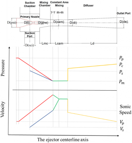
Figures 3 and 4 depict the theoretical pressure and velocity distribution at the ejector centerline of critical and subcritical modes. The flow description on the h-s diagram is shown in Figure 5, There are four major pressures to consider (primary, secondary, mixing, and condenser). The primary flow enters the primary nozzle at primary pressure, then expands and reduces in pressure as it passes down the nozzle's throat at point (ts), but due to the irreversibility and the entropy increment the flow departs at point (t) while the flow continues to section (y-y), and the pressure of the flow dropped to pressure mixing (Pm), if the primary flow expands ideally it should be at point (pys) but for the irreversibility, it deviates and becomes at point (py), on the other hand, the secondary flow enters from the secondary port with pressure (Ps) and due to the expansion, the pressure slumped to the mixing pressure (Pm) and start the mixing process with the primary flow at section (y-y). The mixed flow completes the process at section (m-m) at the pressure level (Pm). The mixed flow moves to the diffuser inlet while the pressure is augmented excessively from (Pm) level to condenser pressure (Pc), by the same concept of irreversibility the diffuser exit properties swerve from (des) to (de).
Double Choking Case (Critical Mode)
$\mathrm{M}_{\mathrm{t}}$ and $\mathrm{M}_{\mathrm{sy}}=1$
Figure 3. Pressure and velocity distribution (Critical mode)
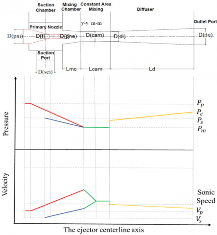
Single Choking Case (Subcritical Mode)
$\mathrm{M}_{\mathrm{t}}=1$ and $\mathrm{M}_{\mathrm{sy}}<1$
Figure 4. Pressure and velocity distribution (sub-critical mode)
The flow description on the h-s diagram is shown in Figure 5.
Figure 5. (h-s) diagram for ejector theoretical operational procedure
3.3 The model parameters
$P_p, T_p, P_s, T_s, P_c, T_c$
$\eta_p, \eta_{p y}, \eta_s, \eta_d, \psi_m$
$d_{p i}, d_{s c i}, d_t, d_{p n e}, d_{c a m}, d_{d i}, d_{d e}, L_{m c}, L_m, L_d$
Cross-section areas of the ejectors
$\left(A_{\mathrm{t}}, A_{\text {pne }}, A_{\mathrm{mc}}\right.$, and $\left.A_{\text {cam }}\right)=\frac{\pi}{4} \mathrm{~d}^2$ (5)
Area ratio $(\mathrm{AR})=\frac{A_{\text {cam }}}{A_t}$ (6)
From Pp & x=1, it is obtained (sp, hp & ρp)
From Ps & x=1, it is obtained (ss, hp & ρs)
All gas dynamics equations were extracted and adopted to build the model [16].
From the primary nozzle inlet to the throat
If the ejector operates in subcritical mode or critical mode, Mt=1, applying the gas dynamics law gives an expression for the relation between pressures as Eq. (7):
$\frac{P_p}{P_t}=\left[1+\frac{\gamma-1}{2} M_t^2\right]^{\frac{\gamma}{\gamma-1}}$ (7)
For the isentropic process between the primary inlet and nozzle throat, the entropy is obtained from the following relation:
$s_p=s_t$
The isentropic enthalpy at the throat is provided by the following function:
$h_{t_s}=f\left(P_t, s_t\right)$
The isentropic efficiency of the primary nozzle is calculated from Eq. (8):
$\eta_p=\frac{h_p-h_t}{h_p-h_{t_s}}$ (8)
The primary flow velocity at the throat is obtained by applying the conservation of energy, with the velocity calculated from Eq. (9):
$u_t=\sqrt{2\left(h_p-h_t\right)}$ (9)
The primary mass flowrate is calculated from Eq. (10):
$\dot{m}_p=\rho_t A_t u_t$ (10)
From primary nozzle throat to section y-y
For the isentropic expansion process between the primary inlet and section y-y, it is obtained from the following relation:
$s_p=s_{p y}$
The isentropic enthalpy for primary flow at section y-y is given by:
$h_{p y_s}=f\left(s_{p y}, P_{p y}\right)$
The isentropic efficiency of the primary flow at section y-y is calculated from Eq. (11):
$\eta_{p y}=\frac{h_t-h_{p y}}{h_t-h_{p y_s}}$ (11)
From secondary inlet to section y-y
The isentropic entropy for secondary flow at section y-y is obtained from the following relation:
$s_s=s_{s y}$
The isentropic enthalpy for secondary flow at section y-y is obtained from the following relation:
$h_{s y s}=f\left(s_{s y}, P_{s y}\right)$
The isentropic efficiency of secondary flow is calculated from Eq. (12):
$\eta_s=\frac{h_s-h_{s y s}}{h_s-h_{s y}}$ (12)
The density of the flow at the secondary flow is extracted as:
$\rho_{s y}=f\left(h_{s y}, P_{s y}\right)$
The velocity of the secondary flow at section y-y is obtained by applying the conservation of energy, with the velocity calculated from Eq. (13):
$u_{s y}=\sqrt{2\left(h_s-h_{s y}\right)}$ (13)
From the primary nozzle exit continues to section y-y
By applying the gas dynamics relation between the area ratio and Mach number we obtain Eq. (14):
$\left(\frac{A_{p n e}}{A_t}\right)^2=\left(\frac{1}{M_{p n e}^2}\right)\left[\left(\frac{2}{\gamma+1}\right)\left(1+\left(\frac{\gamma-1}{2}\right) M_{p n e}^2\right)\right]^{\frac{\gamma+1}{\gamma-1}}$ (14)
By applying the relationship between pressure ratio and Mach number, we obtain Eq. (15):
$\frac{P_p}{P_{p n e}}=\left[1+\frac{\gamma-1}{2} M_{p n e}^2\right]^{\frac{\gamma}{\gamma-1}}$ (15)
Similarly, considering the relation between pressure ratio and Mach number at the primary nozzle exit and section y-y, it is obtained in Eq. (16):
$\frac{P_{p y}}{P_{p n e}}=\frac{\left[1+\frac{\gamma-1}{2} M_{p n e}^2\right]^{\frac{\gamma}{\gamma-1}}}{\left[1+\frac{\gamma-1}{2} M_{p y}^2\right]^{\frac{\gamma}{\gamma-1}}}$ (16)
By applying the gas dynamics relation between the area ratio and Mach number at the primary nozzle exit and section y-y, it is obtained Eq. (17):
$\frac{A_{p y}}{A_{p n e}}=\frac{\frac{\eta_{p y}}{M_{p y}}\left[\left(\frac{2}{\gamma+1}\right)\left(1+\frac{\gamma-1}{2} M_{p y}^2\right)\right]^{\frac{\gamma+1}{2(\gamma-1)}}}{\frac{1}{M_{p n e}}\left[\left(\frac{2}{\gamma+1}\right)\left(1+\frac{\gamma-1}{2} M_{p n e}^2\right)\right]^{\frac{\gamma+1}{2(\gamma-1)}}}$ (17)
The calculation for the entrainment ratio
If the ejector is in critical mode, it is assumed Msy=1, and if the ejector is in sub-critical mode, it is assumed Msy<1.
By applying the relationship between pressure ratio and Mach number to the secondary inlet and critical pressure at section y-y, it is obtained Eq. (18):
$P_s=P_{s y_{\text {critical }}}\left[1+\left[\frac{\gamma-1}{2}\right] M_{s y}^2\right]^{\frac{\gamma}{\gamma-1}}$ (18)
where, Asy and Apy can be found in Eq. (19) below, given Acam:
$A_{c a m}=A_{p y}+A_{s y}$ (19)
The secondary mass flow rate is given by Eq. (20):
$\dot{m}_s=\rho_{s y} u_{s y} A_{s y}$ (20)
The entrainment ratio is given by Eq. (21):
$\omega_{t h}=\frac{\dot{m}_s}{\dot{m}_p}$ (21)
From mixed flow at section y-y to section m-m
Applying the principles of conservation of momentum and energy to the flow in the mixing chamber at section y-y and section m-m.
The mixing efficiency is a non-dimensional parameter to measure the quality of the mixing process as shown in Eq. (22):
$\psi=\frac{u_m^2}{u_{m_{\text {ideal }}^2}}$ (22)
By applying the conservation of momentum, it is obtained Eqn. (23):
$\sqrt{\psi_m}\left(\dot{m}_p u_{p y}+\dot{m}_s u_{s y}\right)=\left(\dot{m}_s+\dot{m}_p\right) u_m$ (23)
To simplify, the secondary flow velocity is neglected at section y-y compared to that of the primary flow and divide Eq. (24) by $\dot{m}_p$:
$\sqrt{\psi_m}\left(u_{p y}\right)=(\omega+1) u_m$ (24)
The conservation of energy at constant area mixing region obtained as Eq. (25):
$\dot{m}_p\left[h_{p y}+\frac{u_{p y}^2}{2}\right]+\dot{m}_S\left[h_{s y}+\frac{u_{s y}^2}{2}\right]=\left(\dot{m}_s+\dot{m}_p\right)\left[h_m+\frac{u_m^2}{2}\right]$ (25)
Similarly, simplify Eq. (24) by neglecting the secondary flow velocity at section y-y compared to the primary flow and dividing Eq. (25) by $\dot{m}_p$:
$\left[h_{p y}+\frac{u_{p y}^2}{2}\right]+\omega\left[h_{s y}\right]=(\omega+1)\left[h_m+\frac{u_m^2}{2}\right]$ (26)
The mixing point entropy, sm, is given as the following function:
$s_m=f\left(h_m, P_m\right)$
Mixed flow from section m-m to the diffuser inlet
Neglecting any change in enthalpy between section m-m and the diffuser inlet, the enthalpy at the inlet to the diffuser is expressed as the following:
$h_{d i}=h_m$
The isentropic efficiency of the diffuser was obtained as Eq. (27):
$\eta_d=\frac{h_{d e_s}-h_{d i}}{h_{d e}-h_{d i}}$ (27)
where, $h_{d e_s}=f\left(P_c, s_{d i}\right)$.
The local sound speed is obtained from the properties of the refrigerant as the following function:
$a_m=f\left(P_m, x=1\right)$
The Mach number at the mixing point is obtained from Eq. (28):
$M_m=\frac{u_m}{a_m}$ (28)
The Mach number at the diffuser inlet is obtained from Eq. (29):
$M_{d i}^2=\frac{1+\left[\frac{\gamma-1}{2}\right] M_m^2}{\gamma M_m^2-\left[\frac{\gamma-1}{2}\right]}$ (29)
By applying the relationship between pressure ratio and Mach number between section m-m and diffuser inlet, a length of the constant area, we obtain Eq. (30):
$\frac{P_{d i}}{P_m}=\left(1+2\left(M_m^2-1\right)\left[\frac{\gamma}{\gamma+1}\right]\right)$ (30)
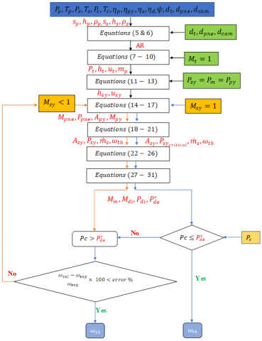
Figure 6. Flowchart of the mathematical model procedure
Diffuser inlet to (ejector outlet/condenser inlet)
Applying the relationship between pressure ratio and Mach number at the diffuser inlet and exit it is obtained Eq. (31):
$\frac{P_{d e}^*}{P_{d i}}=\left[1+\left[\frac{\gamma-1}{2}\right] M_{d i}^2\right]^{\frac{\gamma}{\gamma-1}}$ (31)
where, $P_{d e}^*$ compared to condenser pressure Pc.
The mathematical model procedure is summarized in the flow chart in Figure 6.
4.1 The mathematical model – validation results
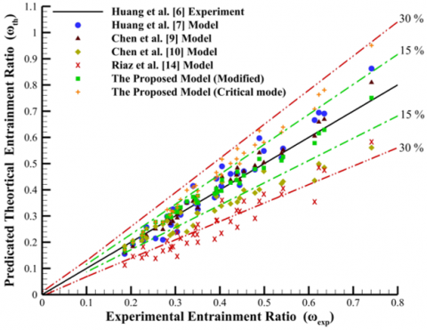
The mathematical model’s validation process started by comparing the results obtained with previously published experimental data in study of Huang et al. [6] and other model predictions in the earlier studies [7, 9, 10, 14], see Figures 7 and 8.
The current model started with the assumption that the ejector operated in the critical mode for all its working conditions and compared the diffuser exit pressure $\left(P_{d e}^*\right)$ with the condenser back pressure $\left(P_c\right)$, if $\left(P_{d e}^* \geq P_c\right)$ so the model calculates the entrainment ratio, if $\left(P_{d e}^*<P_c\right)$, the model calculates the error and then checks the value whether it is in the range ± 20% the model computes the entrainment ratio if the error is outside the range, Then the modified model, the subcritical mode, obtained by varying the Mach number of the secondary flow through section y-y by trial and error to the values below the sonic condition until it was within an acceptable error (± 20%) of the experimental data, While the critical mode overestimating the entrainment ratio, the modified model showed good agreement with the published data (maximum error = 9.85%).
Figure 7. The comparison between the published entrainment ratio results and the proposed model
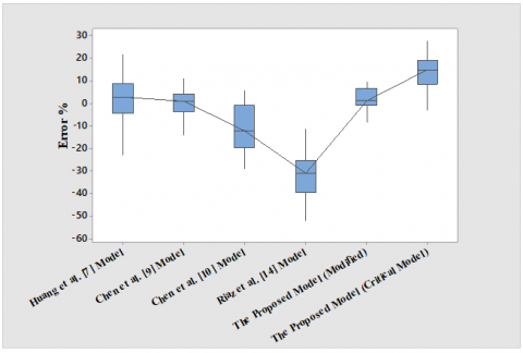
It has been noted that among the published models, Riaz et al. [14] most underestimated the experimental results. The model closest to the published experimental data were those of Chen et al. [9] and the modified model introduced here, those findings are supported by the comparison of the average for the six models and the error range.
Figure 8. The comparison between the averages of six models
4.2 Statistical analysis of the mathematical models
Statistical analysis was conducted on the extracted results from the mathematical model, the objective of the analysis was to test if the new proposal has a significant effect on the output results or if it is minor.
ANOVA is a statistical test that detects whether there are statistically significant differences between the means of three or more independent groups [17]. If the test is applied to three sets of data (a, b, and c) there are two hypotheses: the null hypothesis, the means of the groups are equal Ha: μa= μb=μc, and the alternative hypothesis that the means are not equal Ho: μa≠ μb≠μc. Here the confidence level was set as 95%.
(P- value) represents the probability value of the statistical sample if the null hypothesis is true, while (α) represents the level of significance and it means the probability of rejecting the null hypothesis.
Null hypothesis: the results of the mathematical model are not statistically significantly different from the experimental results, P>α=0.05.
Alternative hypothesis: the results of the mathematical model are statistically significantly different from the experimental results, P<α=0.05.
When comparing two sets of sample data, the larger the F-value the more unlikely it is that the two sets were from the same population.
The predictions of five models were compared with the corresponding experimental results. Because ANOVA tested only one factor, the effect of the mathematical model on the results, one-way ANOVA was suitable. The test results are summarized in Table 1.
The results show clearly that two of the five models deviated significantly from the experimental results (Chen et al. [10] and Riaz et al. [14]. The highest F-value went to Riaz et al. [14] which means the variance within these results was significantly higher than the variance across the groups. While three models produced a null hypothesis at the 5% level, the two which produced results closest to the experimental data were Chen et al. [9] and the modified model proposed here. Chen et al. [9] have the lowest F-value and highest P value showing that this model’s predictions were closest to the measured data. However, the assumptions underpinning this model are very different from the model proposed here, in particular, the refrigerant properties (the assumption that the gas was ideal) while the proposed model works on real gas properties. The proposed relatively simple models show acceptable success and increase the confidence to use such models to calculate the entrainment ratio of the ejector rather than other complex methods.
Table 1. ANOVA test results for the five different models
|
Model |
F-value |
P-value |
Hypothesis testing decision |
|
Huang et al. [7] |
0.17 |
0.6770 |
Accept null |
|
Chen et al. [9] |
0.03 |
0.8640 |
Accept null |
|
Chen et al. [10] |
3.89 |
0.0495 |
Reject null |
|
Riaz et al. [14] |
20.24 |
0.00002 |
Reject null |
|
The proposed model (modified) |
0.05 |
0.8320 |
Accept null |
4.3 Comparison with Yan’s experimental results
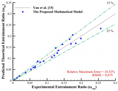
The model validation against Yan et al. [15] experimental results is shown in Figure 9.
Figure 9. The mathematical model predication results against Yan’s experimental data
An ANOVA test was conducted to compare the modified model with Yan’s experimental results as shown in Table 2.
Table 2. ANOVA test results for the five different models
|
F-value |
P-value |
Hypothesis testing decision |
|
0.00459 |
0.946 |
Accept null |
The modified model proposed here when compared with the experimental results obtained by Yan et al. [15] produced a null hypothesis with P=.946>.05 which means there was no significant difference between the predicted results and the experimental data. The small F-value confirmed, to a high degree of confidence, that the two sets of data could both have come from the same population.
4.4 Empirical relationship by using the regression model
By using the experimental results of Huang et al. [6], a regression model was created. The resultant equation included the input operating conditions (Pp, Ps, and Pc) and one of the most important of the geometry parameters, the area ratio (AR). The regression was assumed to be linear to create the regression model, the Pearson correlation test was established to illustrate the inputs that most affected the experimental data output.
The input and output pressures can be combined as shown in Eqns. (32)-(33):
Compression Ratio (CR):
$\beta=\frac{P_c}{P_s}$ (32)
Expansion Ratio (ExR):
$\lambda=\frac{P_p}{P_s}$ (33)
The values of the Pearson correlation between pressure ratios and temperature ratios show that both variables are highly correlated to each other, see Table 3. Thus, input temperatures were omitted from the regression model due to their being effectively included with the pressures.
Table 3. Pearson correlation between pressure ratios and temperature ratios
|
Variables |
Pearson correlation |
Result |
|
$\frac{T_p}{T_s}$ and $\frac{P_p}{P_s}$ |
0.989 |
Strongly positively correlated |
|
$\frac{T_c}{T_s}$ and $\frac{P_c}{P_s}$ |
0.995 |
Strongly positively correlated |
Table 4. Pearson correlation of the independent variables AR, CR, and ExR with the dependent variable ω
|
Variable |
Pearson correlation Coeff. |
Result |
|
Area ratio (AR) |
0.648 |
Positively correlated |
|
Compression ratio (CR) |
-0.947 |
Negatively correlated |
|
Expansion ratio (ExR) |
-0.658 |
Negatively correlated |
Pearson correlations of area ratio (AR), compression ratio (CR), and expansion ratio (ExR) with entrainment ratio (ω) are summarized in Table 4. The results show CR and ExR are negatively correlated with the entrainment ratio while AR is positively correlated.
4.5 The regression model for the experimental results
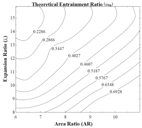
Figure 10 presents the effect of the expansion ratio and area ratio on the entrainment ratio. The results show that for a fixed expansion ratio, the entrainment ratio increases with the area ratio, whereas if the ejector has a fixed area ratio, and entrainment ratio decreases as the expansion ratio increases.
Figure 11 demonstrates the effect of compression ratio and area ratio on the entrainment ratio. The results show that at a fixed compression ratio, the entrainment ratio tends to increase as the area ratio increases, whereas, for a fixed area ratio, the entrainment ratio tends to decrease with an increase in the expansion ratio.
Figure 10. The results of entrainment ratio (ω) as a function of expansion ratio (λ) and area ratio (AR)
Figure 11. The results of entrainment ratio (ω) as a function of compression ratio (β) and area ratio (AR)
From the results shown in Figures 10 and 11, we see the relationships between the ejector performance parameters and entrainment ratio are nonlinear. The operating conditions (compression ratio and expansion ratio) are inversely related to the entrainment ratio while the geometric parameter (area ratio) affected it positively.
The general multiple regression equation with three independent variables can be expressed as mentioned in the study [18] and it is described in Eq. (34):
$\hat{\mathrm{Y}}=a+b_1 x_1^2+b_2 x_1 x_2+b_3 x_1 x_3+b_1 x_1 x_2+b_2 x_2^2+b_3 x_2 x_3+b_1 x_1 x_3+b_2 x_2 x_3+b_3 x_3^2$ (34)
The regression model is represented by Eq. (35):
$\omega_{\exp _r}=0.0000154+0.0039(A R)^2-0.0031(A R \times \lambda)+0.0047(A R \times \beta)+0.0039(A R \times \lambda)-0.0031\left(\lambda^2\right)+0.0047(\lambda \times \beta)$
$+0.0039(A R \times \beta)-0.0031(\lambda \times \beta)+0.0047\left(\beta^2\right)$ (35)
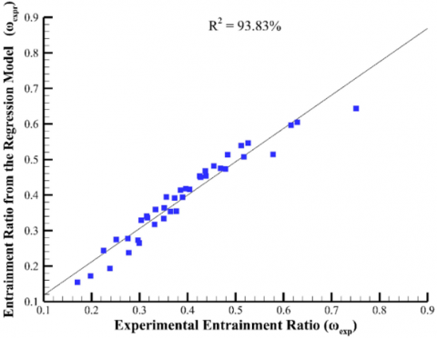
The regression model equation shows a good agreement with the experimental results with the coefficient of determination, R2=0.9383 which means approximately 93.83% of the observed variation can be explained by the model. Thus, the regression model is a very good fit for the experimental results, see Figure 12.
This regression model is valid for the values of area ratios and operating conditions range mentioned in Huang et al. [6] experimental results.
Figure 12. Regression model and experimental data
4.6 Case study – conventional ejector refrigeration system
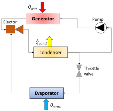
A case study was conducted to test the effect of ejector performance parameters on the system COP. The study was of a single ejector refrigeration cycle operated with R134a. A schematic of the basic design is shown in Figure 13.
Figure 13. Schematic of conventional ejector refrigeration cycle
$\mathrm{COP}=\frac{\dot{\mathrm{Q}}_{\mathrm{evap}}}{\dot{\mathrm{Q}}_{g e n}}=\frac{\dot{\mathrm{m}}_{\mathrm{s}}\left(\mathrm{he}_{\mathrm{o}}-\mathrm{he}_{\mathrm{i}}\right)}{\dot{\mathrm{m}}_{\mathrm{p}}\left(\mathrm{hg}_o-\mathrm{hg}_{\mathrm{i}}\right)}=\omega \frac{\left(\mathrm{h}_{\mathrm{e}_{\mathrm{o}}}-\mathrm{h}_{\mathrm{e}_{\mathrm{i}}}\right)}{\left(\mathrm{h}_{\mathrm{g}_0}-\mathrm{h}_{\mathrm{g}_{\mathrm{i}}}\right)}$ (36)
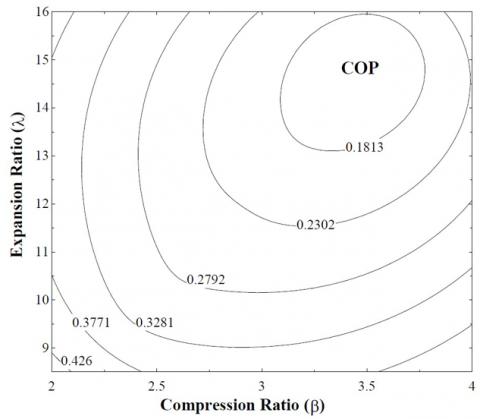
Figure 14 represents the relationship between ejector performance parameters (expansion and compression ratios) with refrigeration system COP for a fixed area ratio, AR=6.44. The results demonstrate that at the same expansion ratio, increasing the compression ratio will influence the system’s COP adversely. Similarly increasing the expansion ratio at a fixed compression ratio will also adversely affect the system’s COP.
Figure 14. COP as a function of Expansion ratio (λ) and Compression ratio (β) at AR=6.44
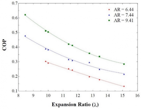
Figure 15. COP as a function of Expansion ratio (λ) for three values of AR
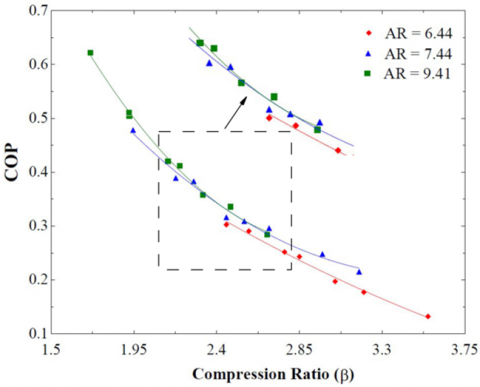
Figure 16. COP as a function of compression ratio (β) for three values of AR
Figure 15 illustrates the relationship between the expansion ratio and COP for three values of the area ratio. Increasing the expansion ratio decreases the COP for all values of the AR, though the higher the AR the greater the value of the COP. Similarly in Figure 16, increasing the compression ratio reduced the value of the COP though, again, the higher the AR the greater the value of the COP.
|
Acronyms |
|
|
ANOVA |
Analysis of variance |
|
AR |
Area ratio |
|
CAM |
Constant area mixing |
|
COP |
Coefficient of Performance |
|
CPM |
Constant pressure mixing |
|
CRMC |
Constant rate of momentum change |
|
Symbols |
|
|
Cp |
The heat capacity at constant pressure (kJ/mol K) |
|
E |
Energy (kJ) |
|
h |
Enthalpy (kJ/kg) |
|
$\dot{m}$ |
Mass flowrate (kg/s) |
|
M |
Mach number |
|
P |
Pressure (Pa) |
|
$\dot{Q}$ |
Heat (kW) |
|
R |
Coefficient of determination |
|
s |
Entropy (kJ/ kg K) |
|
T |
Temperature (℃) |
|
u |
Velocity (m/s) |
|
$\dot{W}$ |
Power (kW) |
|
Greek letters |
|
|
α |
The level of significance |
|
β |
Compression ratio |
|
γ |
Heat capacity ratio |
|
η |
Isentropic efficiency |
|
keff |
Thermal conductivity (kW/m K) |
|
λ |
Expansion ratio |
|
μ |
Mean |
|
μeff |
The effective molecular dynamic viscosity (Pa s) |
|
ρ |
Density (kg/m3) |
|
τij |
Stress tensor |
|
$\hat{Y}$ |
Dependent variable |
|
x |
Independent variable |
|
ψ |
Mixing efficiency |
|
ω |
Entrainment ratio |
|
Subscripts |
|
|
c |
Condenser |
|
cam |
Constant area mixing |
|
d |
Diffuser |
|
de |
Diffuser exit |
|
di |
Diffuser inlet |
|
ei |
Evaporator inlet |
|
eo |
Evaporator outlet |
|
evap |
Evaporator |
|
expr |
Experimental regression |
|
gi |
Generator inlet |
|
go |
Generator outlet |
|
gen |
Generator |
|
m |
Refer to section (m-m) |
|
mc |
Mixing chamber |
|
p |
Primary |
|
pne |
Primary nozzle exit |
|
pni |
Primary nozzle inlet |
|
s |
Secondary |
|
sci |
Secondary inlet |
|
t |
Throat |
|
th |
Theoretical |
|
y |
Refer to section (y-y) |
[1] Keenan, J.H., Neumann, E.P. (1942). A simple air ejector. Journal of Applied Mechanics, 9(2): A75-A81. https://doi.org/10.1115/1.4009187
[2] Keenan, H., Neumann, P., Lustwerk, F. (1950). An investigation of ejector design by analysis and experiment. Journal of Applied Mechanics, 17(3): 299-309. https://doi.org/10.1115/1.4010131
[3] Pianthong, K., Seehanam, W., Behnia, M., Sriveerakul, T., Aphornratana, S. (2007). Investigation and improvement of ejector refrigeration system using computational fluid dynamics technique. Energy Conversion and Management, 48(9): 2556-2564. /https://doi.org/10.1016/j.enconman.2007.03.021
[4] Eames, I.W. (2002). A new prescription for the design of supersonic jet-pumps: The constant rate of momentum change method. Applied Thermal Engineering, 22(2): 121-131. https://doi.org/10.1016/S1359-4311(01)00079-5
[5] Munday, J.T., Bagster, D.F. (1977). A new ejector theory applied to steam jet refrigeration. Industrial & Engineering Chemistry Process Design and Development, 16(4): 442-449. https://doi.org/10.1021/i260064a003
[6] Huang, B.J., Chang, J.M., Wang, C.P., Petrenko, V.A. (1999). A 1-D analysis of ejector performance. International Journal of Refrigeration, 22(5): 354-364. https://doi.org/10.1016/S0140-7007(99)00004-3
[7] Huang, B.J., Chang, J.M. (1999). Empirical correlation for ejector design. International Journal of Refrigeration, 22(5): 379-388. https://doi.org/10.1016/S0140-7007(99)00002-X
[8] Zhu, Y., Cai, W., Wen, C., Li, Y. (2007). Shock circle model for ejector performance evaluation. Energy Conversion and Management, 48(9): 2533-2541. https://doi.org/10.1016/j.enconman.2007.03.024
[9] Chen, W., Liu, M., Chong, D., Yan, J., Little, A.B., Bartosiewicz, Y. (2013). A 1D model to predict ejector performance at critical and sub-critical operational regimes. International Journal of Refrigeration, 36(6): 1750-1761. https://doi.org/10.1016/j.ijrefrig.2013.04.009
[10] Chen, J., Havtun, H., Palm, B. (2014). Investigation of ejectors in refrigeration system: Optimum performance evaluation and ejector area ratios perspectives. Applied Thermal Engineering, 64(1-2): 182-191. https://doi.org/10.1016/j.applthermaleng.2013.12.034
[11] Shi, C., Chen, H., Chen, W., Zhang, S., Chong, D., Yan, J. (2015). 1D model to predict ejector performance at critical and sub-critical operation in the refrigeration system. Energy Procedia, 75: 1477-1483. https://doi.org/10.1016/j.egypro.2015.07.271
[12] Saleh, B. (2016). Performance analysis and working fluid selection for ejector refrigeration cycle. Applied Thermal Engineering, 107: 114-124. https://doi.org/10.1016/j.applthermaleng.2016.06.147
[13] Chen, W., Shi, C., Zhang, S., Chen, H., Chong, D., Yan, U. (2017). Theoretical analysis of ejector refrigeration system performance under overall modes. Applied Energy, 185: 2074-2084. https://doi.org/10.1016/j.apenergy.2016.01.103
[14] Riaz, F., Lee, P.S., Chou, S.K. (2020). Thermal modelling and optimization of low-grade waste heat driven ejector refrigeration system incorporating a direct ejector model. Applied Thermal Engineering, 167: 114710. https://doi.org/10.1016/j.applthermaleng.2019.114710
[15] Yan, J., Cai, W., Li, Y. (2012). Geometry parameters effect for air-cooled ejector cooling systems with R134a refrigerant. Renewable Energy, 46: 155-163. https://doi.org/10.1016/j.renene.2012.03.031
[16] Zucker, R.D., Biblarz, O. (2019). Fundamentals of Gas Dynamics. John Wiley & Sons.
[17] Watkins, J.C. (2017). An introduction to the science of statistics: Preliminary edition. Technometrics, 46(3): 371-372.
[18] Evenson, P. (1978). Calculation of multiple regression with three independent variables using a programable pocket calculator. Agricultural Experiment Station Technical Bulletins, 55. http://openprairie.sdstate.edu/agexperimentsta_tb.