Kolli Vijaya| Bommanna Lavanya*
© 2022 IIETA. This article is published by IIETA and is licensed under the CC BY 4.0 license (http://creativecommons.org/licenses/by/4.0/).
OPEN ACCESS
The overall exploration is excited to investigate the MHD limit layer float of a nanofluid with the results of attractive field, slip limit situation, warm radiation and synthetic reaction has been researched. Closeness change is utilized to change over the administering non-straight limit layer conditions into coupled better request non-direct normal differential conditions. those conditions are mathematically addressed utilizing fourth request R-k technique alongside shooting strategy. An assessment has been accomplished to explain the outcomes of overseeing boundaries like assorted materially conditions. Mathematical results are gotten for the speed, temperature and mindfulness, as well as, for the pores and skin rubbing, close by Nusselt reach and neighborhood Sherwood range for a few benefits of overseeing boundaries. The mathematical results are talked about through graphically and referenced subjectively.
MHD, heat transfer, mass transfer, nano-fluid, stretching sheet, Brownian motion, thermophoresis
Various examinations in the field of liquid mechanics have been directed utilizing an extended sheet and a limit layer stream with a uniform liquid stream. These are upheld in different industrialized and specialized applications, including metallurgy, polymer expulsion, cooling an unending metallic plate in a cooling shower, the assembling of material and glass filaments, and chilling or drying of papers. The slip stream framework, which utilizes the Navier-Stir up conditions in the limit states of slip speed, temperature, and focus, incorporates miniature and nano-scale fluids. Ullah et al. [1] taken a gander at the substance response and hydrodynamic slip impact on Casson nanofluid's inconsistent electrically directing stream. wedge movement delivering shaky electric conduction. The convection current delivered by hot liquid warms the wedge wall. Acquire in the Casson boundary [2].
Within the sight of pull and infusion, Oladapo Olanrewaju researched the warm dispersion (Soret impact) and dissemination thermo (Dufour) qualities of an electrically directing, incompressible liquid over a past moving vertical plate. For light-to-medium atomic weight liquids (such H2, air), it was noticed that Soret and Dufour impacts as well as pull and infusion boundaries ought to be critical studied by Olanrewaju and Makinde [3].
Makende and Olanrewaju [4] researched the Soret and Dufer impacts for the parallel blending of nth-request Arrhenius type irreversible synthetic response and radiative intensity move impact for shaky blended convection stream that is going through an upward permeable level plate [5]. The Casson nano fluid stream on an extended sheet within the sight of substance response and intensity source/sink was investigated by Kumar et al. [6]. On speed and temperature angles at the limit layer, the meaning of the Marangoni number impact was taken note. The thickness of the warm limit layer diminishes as Lewis number and compound response boundary increment [6]. Within the sight of lightness and a cross over attractive field, Makinde [7] concentrated on the Soret and Dufour impacts for an incompressible Boussinesq liquid across an upward permeable plate (with steady intensity stream). On the plate surface, it was found that nearby skin grinding ascends with higher Ec, M, Sr, Du, and K boundaries and falls with higher Sc values. As Ec, Sc, and different boundaries increment, the neighborhood mass exchange rate declines.
With an ascent in the Ec, Sc, M, Du, K, and Sr esteems, the nearby mass exchange rate drops [7]. On persistently moving level surfaces, Sakiadis [8] explored laminar and tempestuous limit layer conduct. He likewise dissected the peculiarities on account of limited length plates. While tempestuous limit layer conduct must be addressed utilizing necessary methods, laminar limit layer conduct can be tackled utilizing both essential and mathematical methodologies. Speed profiles are utilized as limit conditions in these two systems to handle the issues. In their conversation of the exchange of a thick gas stream between two separating level walls, Brutyan and Krapivsky [9] fostered a condition relating the exchange coefficient to temperature. The wall edge is believed to be temperature subordinate, and the wall surface is believed to be a protector. It makes the progression of gas send heat. This shows that the exchange coefficient and gas stream (the exchange of gas between walls) are elements of temperature.
Misra and Pandey [10] used wave length estimates at various peripheral fluid-flow layer thicknesses to study the flow rate of fluid across interface surfaces under various pressure levels. He noticed that a faster flow rate is caused by a thinner peripheral layer. In a two-dimensional channel, the peristaltic flow of theologically complicated physiological fluids may be studied using the perturbation series approach, as demonstrated by LUCAS [11]. Dash et al. [12] researched the impact of yield stress on Casson fluid flow through a horizontal porous media that is enclosed by a tube.
He observed that in the presence of yield stress the fluid flow is independent of permeability of porous medium [12]. Kashyap et al. [13], the author studied the uniform heat source effect in the presence of first order destructive chemical reaction for MHD UCM fluid while passing through porous media. He observed that heat source cause for the dilation of concentrated fluid and increment in fluid velocity. Also porous slip condition oppose the motion of fluid through the upper surface of porous plate [13]. Gbadeyan et al. [14] studied Dufour and Soret effect for MHD fluid flow passing through a vertical channel which is bounded by flat and wavy walls in the presence of uniform magnetic field. In this case the author used perturbation method.
Using Bation theory, ordinary differential equations may be solved [14]. On a non-linearly stretched sheet implanted in a non-Darcy porous medium, Reddy and Krishna [15] investigated the Soret and Dufour effects on MHD fluid flow. The impacts of the magnetic parameter, the Soret number, the Dufour number, the micro rotation profile, the concentration, the Nusselt number, the skin-friction number, and the Sherwood number are investigated. Singh and Shishodia [16] investigated the impact of magnetic fields on viscous fluids moving via electrical conductors. She found that the homotropy perturbation sumudu transform method (HPSTM) is preferable to the magneto hydrodynamics (MHD) approach for obtaining an accurate solution in this study. Das [17] the issue of heated and electrically conducting MHD fluid flow on a parallelly moving plate was addressed by the author in the numerical solution for the thermal radiation presence utilising the MATLAB BVP solver bvp4c technique. In comparison to other approaches used in earlier study, he found that the MATLAB BVP solver bvp4c method is more appropriate.
Ibukun Sarah and colleagues discovered that the Casson parameter inhibits the increase in temperature and velocity. The Soret parameter raises the fluid concentration whereas the Dufour parameter lowers the flow temperature [18]. Ram and Sharma [19] investigated the effects of ferrofluid flow and MFD viscosity on a rotational disc. They noticed that the MFD viscosity parameters changed depending on the pressure profiles and velocity components of Karman's dimensionless parameter. The effects of non-uniform heat sources and sinks for Carreau and Casson nano fluids on homogeneous and heterogeneous stretching surface media were investigated by the author. He noted that the Casson fluid exhibits higher heat and mass transport rates than the Carreau fluid [20]. The effects of thermophoresis and Brownian motion on MHD radiative Casson fluid travelling through a past-moving 2D wedge containing gyro tactic bacteria were examined by Raju et al. [21] He noticed that in the suction and injection processes, Brownian motion reduces the boundary layer and thermophoresis causes the temperature to rise. Thermophoresis and Brownian motion characteristics cause the Casson fluid to move more quickly and with less temperature, concentration, and density. In two situations, water, silver mixed nano fluids and water, graphene mixed nano fluids with and without micro size dust particle doping, Upadhya et al. [22] evaluated heat transmission and temperature distribution features. He noticed that a water, grapheme mixed nano fluid performed better at transferring heat than a water, silver fluid. The two scenarios' temperature distributions are identical. with thermal relaxation. Hayata et al. [23] investigated the effects of viscosity dissipation, temperature, and thermal conductivity on the thermophoresis and Brownian motion for mixed Casson fluid flow. He noted that for process factors such the Nusslet number, Sherwood number, and Skin friction coefficient, the thermophoresis effect is inverted with respect to the Brownian motion effect for fluid flow. In-depth research on the heat and mass transport properties of natural convective magneto hydrodynamic Casson fluid flow in an unstable situation was conducted by Kataria and Patel [24]. In the non-linear stretching cylinder instance, Hayat et al. [25] found that thermal radiation and magnetic field raise temperature profile and velocity decreases with magnetic field for boundary layer flow viscous fluid. The similar result, where fluid flow velocity decreases with magnetic field, was previously noted by Sarojamma et al. [26]. This behaviour has significant bio-medical uses, notably for studying blood flow in the cardiovascular system.
Consider a 2-D consistent state limit layer stream of a nanofluid overextending sheet within the sight of substance response with surface with ' ' being a steady. The stream is thought to be created by extending sheet giving temperature Tw and focus Cw considering. The extending speed of the sheet is from a slim cut at the beginning. The sheet is extended so that the speed anytime on the sheet becomes corresponding to the separation from the beginning. The encompassing temperature and fixation are $T_{\infty}$ and $C_{\infty}$ separately. The stream is exposed to the joined impact of warm radiation and a cross over attractive field of solidarity B0, which is thought to be applied in the positive y-course, ordinary to the surface, the actuated attractive field is additionally thought to be little contrasted with the applied attractive field; so it is disregarded. It is additionally expected that the base liquid and the suspended nanoparticles are in warm equilibrium. It is picked that the direction framework x-pivot is along extending sheet and y-hub is typical to the sheet. Also it is accepted that there leaves a homogeneous compound response of first request with rate constant between the diffusing species and the liquid.
Under the above suppositions, the overseeing condition of the preservation of mass, force, energy and nanoparticles division within the sight of attractive field and warm radiation past a stretching sheet can be communicated as:
$\frac{\partial u}{\partial x}+\frac{\partial v}{\partial y}=0$ (1)
$u \frac{\partial u}{\partial x}+v \frac{\partial u}{\partial y}=-\frac{1}{\rho_f} \frac{\partial p}{\partial x}+v\left(\frac{\partial^2 u}{\partial x^2}+\frac{\partial^2 u}{\partial y^2}\right)-\frac{\sigma B_0^2}{\rho_f} u$ (2)
$u \frac{\partial v}{\partial x}+v \frac{\partial v}{\partial y}=-\frac{1}{\rho_f} \frac{\partial p}{\partial y}+v\left(\frac{\partial^2 v}{\partial x^2}+\frac{\partial^2 v}{\partial y^2}\right)-\frac{\sigma B_0^2}{\rho_f} v$ (3)
$\begin{aligned} u \frac{\partial T}{\partial x}+v \frac{\partial T}{\partial y}=\alpha & \left(\frac{\partial^2 T}{\partial x^2}+\frac{\partial^2 T}{\partial y^2}\right)-\frac{1}{\rho_f c_f}\left(\frac{\partial q_r}{\partial y}\right) \\ &+\frac{\mu}{\rho c_p}\left(\frac{\partial u}{\partial y}\right)^2+\frac{\sigma B_0^2}{\rho c_p} u^2 \\ &+\tau\left\{D_B\left(\frac{\partial C}{\partial x} \frac{\partial T}{\partial x}+\frac{\partial C}{\partial y} \frac{\partial T}{\partial y}\right)\right. \\ & \left.+\frac{D_T}{T_{\infty}}\left(\left(\frac{\partial T}{\partial x}\right)^2+\left(\frac{\partial T}{\partial y}\right)^2\right)\right\}\end{aligned}$ (4)
$\begin{aligned} u \frac{\partial C}{\partial x}+v \frac{\partial C}{\partial y}=D_B & \left(\frac{\partial^2 C}{\partial x^2}+\frac{\partial^2 C}{\partial y^2}\right) \\ &+\frac{D_T}{T_{\infty}}\left(\frac{\partial^2 T}{\partial x^2}+\frac{\partial^2 T}{\partial y^2}\right)-K_r^1\left(C-C_{\infty}\right)\end{aligned}$ (5)
where, x and y address coordinate tomahawks along the consistent surface toward movement and typical to it separately. u, v means speed of the liquid along x and y headings. T is temperature of the fluid; C is grouping of the fluid.
$\rho_f, v, \sigma, B_0, \alpha, c_f, c_p, q_r, \tau, D_B, D_T, T_{\infty}, K_r{ }^1$ are the thickness of the base liquid, kinematic consistency, electrical conductivity, attractive field, warm diffusivity, explicit intensity limit of liquid, explicit intensity limit of nanoparticle, radiative intensity/transition, proportion of intensity limits, the Brownian dispersion coefficient, thermophoresis dissemination coefficient, the temperature for away from the sheet and substance response rate steady individually. The limit conditions are:
$\begin{aligned} u=u_w+L \frac{\partial u}{\partial y}, v & =V_w, T=T_w+K_1 \frac{\partial T}{\partial y}, \\ C & =C_w+K_2 \frac{\partial C}{\partial y}, a t y=0 . u \\ & \rightarrow U_{\infty}=0, T \rightarrow T_{\infty}, C \rightarrow C_{\infty} a s y \\ & \rightarrow \infty\end{aligned}$ (6)
where, $u_w=a x, T_w=T_{\infty}+b\left(\frac{x}{l}\right)^2, C_w=C_{\infty}+C\left(\frac{x}{l}\right)^2$ .
L, K1 and K2 are the velocity, the thermal and concentration slip factor respectively and when L = K1 = K2 = 0, no-slip condition is recuperated, l is the reference length of a sheet. The abovementioned. limit condition is substantial when x ≤ l which happens extremely close to the cut.
Utilizing a request greatness investigation of the y-course energy condition (typical to the sheet) and the standard limit layer approximations, for example,
$u \gg v$
$\frac{\partial u}{\partial y} \gg \frac{\partial u}{\partial x}, \frac{\partial v}{\partial x}, \frac{\partial v}{\partial y}$ (7)
$\frac{\partial p}{\partial y}=0$
The pressure distribution throughout the boundary layer in the direction normal to the surface (such as an airfoil) remains relatively constant throughout the boundary layer, and is the same as on the surface itself. The thickness of the velocity boundary layer is normally defined as the distance from the solid body to the point at which the viscous flow velocity is 99% of the free stream velocity Directly following and applying the limit layer estimate, the administering conditions are diminished to:
$\frac{\partial u}{\partial x}+\frac{\partial v}{\partial y}=0$ (8)
$u \frac{\partial u}{\partial x}+v \frac{\partial u}{\partial y}=v\left(\frac{\partial^2 u}{\partial y^2}\right)-\frac{\sigma B_0^2}{\rho_f} u$ (9)
$\begin{aligned} u \frac{\partial T}{\partial x}+v \frac{\partial T}{\partial y}=\alpha( & \left.\frac{\partial^2 T}{\partial y^2}\right)-\frac{1}{\rho_f c_f}\left(\frac{\partial q_r}{\partial y}\right) \\ &+\frac{\mu}{\rho c_p}\left(\frac{\partial u}{\partial y}\right)^2+\frac{\sigma B_0^2}{\rho c_p} u^2 \\ &+\tau\left\{D_B \frac{\partial C}{\partial y} \frac{\partial T}{\partial y}+\frac{D_T}{T_{\infty}}\left(\frac{\partial T}{\partial y}\right)^2\right\}\end{aligned}$ (10)
$u \frac{\partial C}{\partial x}+v \frac{\partial C}{\partial y}=D_B \frac{\partial^2 C}{\partial y^2}+\frac{D_T}{T_{\infty}} \frac{\partial^2 T}{\partial y^2}-K_r^1\left(C-C_{\infty}\right)$ (11)
The boundary conditions are:
$\begin{aligned} u=u_w+L \frac{\partial u}{\partial y}, v & =V_w, T=T_w+K_1 \frac{\partial T}{\partial y}, C \\ &=C_w+K_2 \frac{\partial C}{\partial y}, \text { aty }=0 . u \rightarrow U_{\infty} \\ &=0, T \rightarrow T_{\infty}, C \rightarrow C_{\infty} a s y \rightarrow \infty\end{aligned}$ (12)
where, $\alpha=\frac{k}{(c \rho)_f}, \tau=\frac{(c \rho)_p}{(c \rho)_f}, v=\frac{\mu}{\rho_f}$ ; k is the thermal conductivity coefficient, (cρ)p, (cρ)f are the successful intensity limit of a nano-molecule, compelling intensity limit of liquid.
Presenting the accompanying dimensionless amounts, the numerical examination of the issue is streamlined by utilizing likeness changes:
$\eta=\sqrt{\frac{a}{v}} y, \psi=\sqrt{a v} x f(\eta), \theta(\eta)=\frac{T-T_{\infty}}{T_w-T_{\infty}}, \varphi(\eta)$ $=\frac{C-C_{\infty}}{C_w-C_{\infty}}$ (13)
The condition of progression is fulfilled in the event that a Stream capability is picked as for $\psi(x, y)$ :
$u=\frac{\partial \psi}{\partial y} ; v=-\frac{\partial \psi}{\partial x}$ (14)
The radiative intensity motion in the x-course is thought of as irrelevant when contrasted with y-heading. Consequently by involving Rosseland estimate for radiation, the radiative intensity transition $q_r$ is given by:
$q_r=-\frac{4 \sigma^*}{3 k^*} \frac{\partial T^4}{\partial y}$ (15)
where, $\sigma^*$ and $k^*$ are the Stefan-Boltzmann constant and the mean absorption coefficient, respectively. We assume that the temperature distance within the flow is sufficiently small such that the term T4 may be expressed as a linear function of temperature. This is done by expanding T4 in a Taylor series about a free stream temperature T∞ as follows:
$T^4=T_{\infty}^4+4 T_{\infty}^3\left(T-T_{\infty}\right)+6 T_{\infty}^2\left(T-T_{\infty}\right)^2+\ldots \ldots \ldots$ (16)
Neglecting the higher- order terms in the above equation we get:
$T^4 \cong 4 T_{\infty}^3 T-3 T_{\infty}^4$ (17)
Substituting Eq. (17) in Eq. (15), we get:
$q_r=-\frac{16 T_{\infty}^3 \sigma^*}{3 k^*} \frac{\partial T}{\partial y}$ (18)
Utilizing the likeness change amounts, the overseeing Eqns. (8)-(11) are changed to customary differential conditions as follows:
$f^{\prime \prime \prime}+f f^{\prime \prime}-f^{\prime 2}-M f^{\prime}=0$ (19)
$\left(1+\frac{4 R}{3}\right) \theta^{\prime \prime}+P_r f \theta^{\prime}-2 P_r f^{\prime} \theta+P_r E_c f^{\prime \prime 2}+P_r M E_c f^{\prime 2}+P_r N_b \varphi^{\prime} \theta^{\prime}+P_r N_t \theta^{\prime 2}=0$ (20)
$\varphi^{\prime \prime}+\operatorname{Lef} \varphi^{\prime}-2 L e f^{\prime} \varphi+\frac{N_t}{N_b} \theta^{\prime \prime}-K_r L e \varphi=0$ (21)
The transformed boundary conditions are:
$\begin{aligned} f(0)=S, f^{\prime}(0) =1+a_1 f^{\prime \prime}(0), \theta(0) \\ =1+a_2 \theta^{\prime}(0), \varphi(0) \\ =1+a_3 \varphi^{\prime}(0) a t \eta=0 \\ f^{\prime}(\infty)=0, \theta(\infty) & =0, \varphi(\infty)=0 a s \eta \rightarrow \infty\end{aligned}$ (22)
where, the overseeing actual boundaries are characterized as follows:
$\begin{aligned} & P_r=\frac{v}{\alpha} ; E_c=\frac{u_w^2}{c_p\left(T_w-T \infty\right)} ; R=\frac{4 \sigma^* T_{\infty}^3}{k^* k} M \\ &=\frac{\sigma B_0^2}{\rho_f a} ; N_b \\ &=\frac{\rho_p c_p D_B\left(C_w-C_{\infty}\right)}{\rho_f c_f v} ; N_t \\ &=\frac{\rho_p c_p D_T\left(T_w-T_{\infty}\right)}{\rho_f c_f v T_{\infty}} L e=\frac{v}{D_B} ; K_r \\ &=\frac{K_r^1}{a} ; S=\frac{-V_w}{\sqrt{a v}} ; a_1=L \sqrt{\frac{a}{v}} ; a_2 \\ &=K_1 \sqrt{\frac{a}{v}} ; a_3=K_2 \sqrt{\frac{a}{v}}\end{aligned}$ (23)
where, $f^{\prime}, \theta$ and $\varphi$ are the dimensionless velocity, temperature and nanoparticle focus, individually. These are the likeness factors, the prime indicates separation as for $\eta$. $P_r, E_c, R, M, N_b, N_t$, Le $, K_r, S$ denote a Prandtl number, Eckert number, a radiation parameter, magnetic field parameter, a Brownianmotion parameter, a thermophoresis parameter, a Lewis number, chemical reaction parameter, mass suction parameter, respectively.
The significant actual amounts in this issue are neighborhood skin grinding coefficient cf, the local Nusselt number $N u_x$ , and the local Sherwood number Sh are defined as:
$c_f=\frac{\tau_w}{\rho u_w^2}, N u_x=\frac{x q_w}{k\left(T_w-T_{\infty}\right)}, S h_x=\frac{x h_m}{D_B\left(C_w-C_{\infty}\right)}$ (24)
where, the wall heat flux $q_w$ and mass flux $h_m$ are given by:
$q_w=-k\left(\frac{\partial T}{\partial y}\right)_{y=0}, h_m=-D_B\left(\frac{\partial \phi}{\partial y}\right)_{y=0}$ (25)
By using the above equations, we get:
$c_f \sqrt{R e_x}=-f^{\prime \prime}(0), \frac{N u_x}{\sqrt{R e_x}}=-(1+R) \theta^{\prime}(0), \frac{S h_x}{\sqrt{R e_x}}=-h^{\prime}(0) S$ (26)
where, Rex is the local Reynolds number.
A productive fourth request R-K strategy alongside shooting procedure has been utilized to read up the stream model for the above coupled non-straight normal differential conditions (19)-(21) for various benefits of administering boundaries. The non-direct differential conditions are first disintegrated into an arrangement of first request differential condition. The coupled normal differential Eqns. (19)- (21) are third) are third order in f and second order in θ, φ request in which have been diminished an arrangement of seven synchronous conditions for seven questions f one initial condition in each of θ and φ are known. However, the values of f', θ and φ are known at η→∞ To address mathematically this arrangement of Conditions at η=0 utilizing R-K strategy, the arrangement requires seven beginning circumstances yet two starting circumstances in are known. In any case, the upsides of. These end conditions are used to create obscure introductory circumstances at by shooting procedure. The main step of this plan is to pick the suitable worth of. In this manner, to gauge the worth of, we start with some underlying conjecture esteem and take care of the limit esteem issue challenging of Eqns. (19)-(21) to acquire to obtain f″ (0), θ' (0) and φ' (0) The arrangement cycle is rehashed with one bigger worth of until two progressive upsides of contrast solely after wanted huge digit. The last worth is taken as the limited worth of the cut-off for the specific arrangement of actual boundaries for deciding speed, temperature and focus in the limit layer. Subsequent to getting every one of the underlying circumstances we tackle this arrangement of concurrent conditions utilizing fourth request R-K coordination plot. The worth of is chosen to shift from 5 to 20 relying upon the actual boundaries administering the stream so no mathematical wavering would happen. Thus, the coupled boundary value problem of third order in f, second order in θ and φ has been decreased an arrangement of seven synchronous conditions of first request for seven questions as follows lessened a plan of seven simultaneous states of first solicitation for seven inquiries as follows:
$f^{\prime \prime \prime}=-f f^{\prime \prime}+f^{\prime 2}+M f^{\prime}$ (27)
$\theta^{\prime \prime}=-P_r\left(\begin{array}{c}f \theta^{\prime}-2 f^{\prime} \theta+E_c f^{\prime \prime 2}+ \\ \frac{M E_c f^{\prime 2}+N_b \varphi^{\prime} \theta^{\prime}+N_t \theta^{\prime 2}}{1+\frac{4 R}{3}}\end{array}\right)$ (28)
$\varphi^{\prime \prime}=-\operatorname{Lef} \varphi^{\prime}+2 L e f^{\prime} \varphi-\frac{N_t}{N_b} \theta^{\prime \prime}+K_r \operatorname{Le} \varphi$ (29)
We can define a new set of variables as:
$\begin{aligned} f=y_1, f^{\prime}=y_2, & f^{\prime \prime}=y_3, f^{\prime \prime \prime}=y_3^{\prime}, \theta=y_4, \theta^{\prime} \\ &=y_5, \theta^{\prime \prime}=y_5^{\prime}, \varphi=y_6, \varphi^{\prime}=y_7, \varphi^{\prime \prime} \\ &=y_7^{\prime}\end{aligned}$ (30)
The coupled higher solicitation non-straight differential circumstances and the breaking point conditions may be changed to seven indistinguishable first solicitation differential circumstances and cut-off conditions, exclusively as given under:
$y_1^{\prime}=y_2$
$y_2^{\prime}=y_3$
$y_3^{\prime}=-y_1 y_3+y_2^2+M y_2$
$y_4^{\prime}=y_5$
$y_5^{\prime}=-P_r\left(\begin{array}{c}y_1 y_5-2 y_2 y_4+E_c y_3^2+ \\ \frac{M E_c y_2^2+N_b y_5 y_7+N_t y_5^2}{1+\frac{4 R}{3}}\end{array}\right)$ (31)
$y_6^{\prime}=y_7$
$y_7^{\prime}$$=-$ Ley $_1 y_7+2 L e y_2 y_6$$+\frac{N_t}{N_b} P_r\left(\begin{array}{c}y_1 y_5-2 y_2 y_4+E_c y_3^2+ \\ \frac{M E_c y_2^2+N_b y_5 y_7+N_t y_5^2}{1+\frac{4 R}{3}}\end{array}\right)+K_r$ Ley $_6$
Here the prime denote differentiation with respect to η and the boundary conditions are
$\begin{aligned} y_1(0)=S, y_2(0) & =1+a_1 y_3(0), y_4(0) \\ & =1+a_2 y_5(0), y_6(0) \\ & =1+a_3 y_7(0), y_2(\infty)=0, y_4(\infty) \\ &=0, y_6(\infty)=0\end{aligned}$ (32)
In this issue, first the limit esteem issue is changed over into Starting Worth issue (IVP).
Then the IVP is settled by fittingly speculating the missing starting worth involving R-K strategy alongside shooting method for a few of boundaries. The mistake resistance of is utilized. The outcomes acquired are introduced through tables and charts.
This segment intends to attract consideration of specialists to research the impacts of stream control boundaries, for example, compound response boundary, attractive field, pull boundary, speed slip boundary, warm slip boundary, fixation slip boundary, Prandtl number, radiation boundary, Lewis n boundary on the MHD stream of a nanofluid limit layer around a penetrable strain film with slip limit conditions. The Runge-Kutta strategy and the shot methodology are utilized to address the administering conditions, and the subsequent outcomes are satisfactory solutions for the speed field, temperature field, fixation appropriation, skin contact, Nusselt number, and Sherwood number. The speed profiles, temperature profiles, and fixation conveyances in Tables 1 and 2 are utilized to analyze and make sense of the effect of different variables on the stream field.
Table:1 illustrates the values of Nusselt number, Sherwood number and Reynolds number with respect to variation of M, S, a1, Pr, R and Kr. It depicts the good result. Table:2 shows the results of Nusselt number, Sherwood number and Reynolds number with respect to variation of parameters like Le, Nt, Nb, a2 and a3. It shows good agreement with the result.
Figure 1. Influence of velocity depiction for different values of the magnetic field parameter (M)
Figure 2. The impact of temperature depiction for various magnetic field parameter values(M)
Figure 3. The impact of concentration depiction for various magnetic field parameter values(M)
Table 1. Illustrates the values of Nusselt number, Sherwood number and Reynolds number with respect to variation of M, S, a1, Pr, R and Kr
|
M |
S |
a1 |
Pr |
R |
Kr |
Cf |
Nu |
Sh |
|
0 |
1 |
1 |
0.71 |
0.5 |
0.5 |
0.569889 |
0.362559 |
0.527008 |
|
1 |
0.638897 |
0.371891 |
0.529851 |
|||||
|
2 |
0.677815 |
0.386340 |
0.534333 |
|||||
|
3 |
0.704402 |
0.413183 |
0.543188 |
|||||
|
1 |
0 |
1 |
0.71 |
0.5 |
0.5 |
0.546604 |
0.334171 |
1.298560 |
|
0.5 |
0.593810 |
0.384162 |
1.535582 |
|||||
|
1 |
0.638897 |
0.451415 |
1.668027 |
|||||
|
1.5 |
0.679708 |
0.529606 |
1.740455 |
|||||
|
1 |
0.5 |
0 |
0.71 |
0.5 |
0.5 |
0.454208 |
0.356266 |
1.525931 |
|
0.5 |
0.593810 |
0.384162 |
1.535582 |
|||||
|
1 |
0.865753 |
0.429675 |
1.551575 |
|||||
|
1.5 |
1.686142 |
0.526147 |
1.586138 |
|||||
|
1 |
0.5 |
1 |
0.71 |
0.5 |
0.5 |
0.593810 |
0.384162 |
1.475712 |
|
1 |
0.593810 |
0.455057 |
1.482507 |
|||||
|
5 |
0.593810 |
0.829438 |
1.527886 |
|||||
|
7 |
0.593810 |
0.883826 |
1.535582 |
|||||
|
1 |
0.5 |
0,5 |
0.71 |
0.5 |
0.5 |
0.865753 |
0.295251 |
1.551575 |
|
1 |
0.865753 |
0.322920 |
1.558117 |
|||||
|
1.5 |
0.865753 |
0.363767 |
1.562121 |
|||||
|
2 |
0.865753 |
0.429675 |
1.564816 |
|||||
|
1 |
0.5 |
0,5 |
0.71 |
0.5 |
0.5 |
0.865753 |
0.456560 |
1.547534 |
|
1 |
0.865753 |
0.456674 |
1.574690 |
|||||
|
1.5 |
0.865753 |
0.456772 |
1.595737 |
|||||
|
2 |
0.865753 |
0.456858 |
1.613060 |
Table 2. Shows the results of Nusselt number, Sherwood number and Reynolds number with respect to variation of parameters like Le, Nt, Nb, a2 and a3
|
Le |
Nt |
Nb |
a2 |
a3 |
Cf |
Nu |
Sh |
|
1 |
0.865753 |
0.454588 |
0.707984 |
||||
|
1.5 |
0.865753 |
0.454713 |
0.868813 |
||||
|
2 |
0.865753 |
0.454993 |
0.983456 |
||||
|
0.5 |
0.5 |
0.5 |
0.5 |
0.5 |
0.865753 |
0.386080 |
1.112565 |
|
1 |
0.865753 |
0.402798 |
1.204227 |
||||
|
1.5 |
0.865753 |
0.420807 |
1.310076 |
||||
|
2 |
0.865753 |
0.440137 |
1.433525 |
||||
|
0.5 |
0.5 |
0.5 |
0.5 |
0.5 |
0.865753 |
0.392114 |
1.551575 |
|
1 |
0.865753 |
0.404340 |
1.566300 |
||||
|
1.5 |
0.865753 |
0.416860 |
1.571185 |
||||
|
2 |
0.865753 |
0.429675 |
1.573611 |
||||
|
0.5 |
0.5 |
0.5 |
0.5 |
0.5 |
0.865753 |
0.264123 |
1.551575 |
|
1 |
0.865753 |
0.303429 |
1.556040 |
||||
|
1.5 |
0.865753 |
0.356038 |
1.559265 |
||||
|
2 |
0.865753 |
0.429675 |
1.561694 |
||||
|
0.5 |
0.5 |
0.5 |
0.5 |
0.5 |
0.866402 |
0.481812 |
0.460398 |
|
1 |
0.866402 |
0.487951 |
0.601422 |
||||
|
1.5 |
0.866402 |
0.490344 |
0.866987 |
||||
|
2 |
0.866402 |
0.491618 |
1.552512 |
The effect of the magnetic field parameter (M) on the velocity, temperature, and concentration profiles is made clear in Figures 1-3. According to Figure 1, the Lorentz force causes the velocity profiles to drop as the magnetic field value (M) increases. The fluid particles encountered considerable resistance during the travel since it is resistive in nature. As a result, the average speed drops. Figure 2 illustrates how the transverse magnetic field increased the thermal boundary layer's thickness. The thermal boundary layer has increased, although not much. The nanofluid has comparable characteristics to other common fluids in terms of how the magnetic field affects the thermal field. Figure 3 shows that the concentration rises when the magnetic field parameter is increased (M).
The effect of the mass suction parameter (S) on the velocity and concentration profiles is seen in Figures 4 and 5.
The velocity and concentration profiles decrease as the suction parameter (S) value rises. The surface temperature is also decreased, along with the thicknesses of the thermal boundary layer, concentration boundary layer, and concentration boundary layer.
The effect of the velocity slip parameter (a1) on the temperature and concentration profiles is seen in Figures 6 and 7. It is evident that as the values of the velocity slip parameter (a1) grow, so do the profiles of temperature and concentration.
The impact of Prandtl number (Pr) on temperature and concentration profiles is seen in Figures 8 and 9. It is interesting to notice that when temperature rises, the dimensionless Prandtl number (Pr) falls as the concentration of nanoparticles rises. This occurrence is consistent with the idea that the fluid's poor thermal conductivity is linked to its high Pr, which lowers conductivity. As a result, the concentration boundary layer becomes thicker and the thermal boundary layer becomes thinner.
Figure 4. The impact of velocity depiction for various suction parameter values (S)
Figure 5. The impact of concentration depiction for various suction parameter values (S)
Figure 6. The impact of temperature depiction for various velocity slip parameter values (a1)
Figures 10-12 depict how the radiation parameter (R) affects temperature and concentration patterns (11). It is obvious that as the radiation parameter (R) is increased, the temperature profiles rise while the concentration profiles fall. This is brought on by a decrease in the rate of heat transmission at the surface and an increase in the thickness of the thermal boundary layer. The impact of the chemical reaction parameter (Kr) on the concentration profiles is seen in Figure 12. It demonstrates that when the chemical reaction parameter (Kr) increases, the concentration falls.
Figure 7. Concentration depiction effects for various velocity slip parameter values (a1)
Figure 8. Shows the impact of temperature depiction for various Prandtl number values (Pr)
Figure 9. The impact of concentration depiction for various Prandtl number values (Pr)
Figure 13 depicts the variation in Lewis number (Le) on the concentration field. It's interesting to note that both the concentration and the thickness of the concentration boundary layer drop as the Lewis number (Le) rises. This is most likely due to the fact that when the Lewis number rises, the rate of mass transfer does as well. Additionally, it demonstrates that the gradient of concentration at the leaf's surface rises. Additionally, when Le values rise, the concentration on the sheet surface declines.
Figure 10. The impact of temperature depiction for various Radiation parameter values (R)
Figure 11. The impact of concentration depiction for various radiation parameter values (R)
Figure 12. Shows the effects of concentration depiction for various chemical reaction parameter values (Kr)
To see how the thermophoresis parameter (Nt) affects the temperature distribution and concentration field, look at Figures 14 and 15. As a function of the thermophoresis parameter, it has been shown that both temperature and the concentration distribution of nanoparticles rise (Nt). The temperature profile is not significantly affected by rising Nt levels, though. The strength of Nt has a significant impact on the concentration of nanoparticles since the concentration of nanoparticles is a strong function of Nt. Peak values for the concentration of nanoparticles close to the wall show that the volume fraction of nanoparticles at the surface is less than the volume fraction of nanoparticles close to the plate. Finally, it was discovered that the nanoparticles enter into the stretch film as a result of the thermophoresis phenomenon. Additionally, it should be emphasised that when Nt grows, the concentration boundary layer's thickness does as well.
Figure 13. The impact of concentration depiction for various Lewis number values (Le)
Figure 14. Depicts the impact of temperature depiction for various thermophoresis parameter values (Nt)
Figure 15. Shows the impact of concentration depiction for various thermophoresis parameter values (Nt)
Figure 16. Shows the impact of temperature depiction for various Brownian motion parameter values (Nb)
Figure 17. Concentration depiction effects for various Brownian motion parameter values (Nb)
Figure 18. The impact of concentration depiction for various thermal slip parameter values (a2)
The effect of the Brownian motion parameter Nb on the dimensionless profiles of temperature and nanoparticle concentration is seen in Figures 16 and 17. It is noteworthy to see that whereas nanoparticle concentration is a decreasing function of temperature (Nb). This is due to the fact that a nanofluid is a two-phase fluid in which the energy rate is increased by the random movement of nanoparticles. When a result, as the Brownian motion parameter (Nb) rises, so does the temperature. Additionally, it is noted that for lesser Nb, the concentration of nanoparticles peaks near the wall and subsequently declines for greater values of the Brownian motion parameter (Nb).
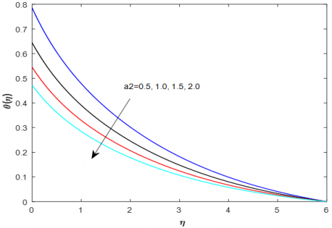
Figures 18 and 19 display the effects of concentration and temperature for various values of the thermal slip parameter (a2) (19). With increasing levels of the thermal slip parameter, it was discovered that both concentration and temperature profiles decreased (a2). Figure 20 displays the impact of different values of the concentration slip parameter on nanoparticle concentration profiles (a3). The concentration profiles are seen to decrease with rising values of the concentration slip parameter (a3).
Figure 19. The impact of temperature depiction for various thermal slip parameter values (a2)
Figure 20. Effect of concentration depiction for various concentration slip parameter values (a3)
The boundary layer MHD nanofluid flow around a permeable tension cylinder with slip boundary conditions was analysed in relation to the impacts of chemical reaction. Tabular presentations of the numerical results were made. Our outcome reveals this.
Creators are appreciative to the arbitrator for the significant ideas who help to work on the nature of this composition and furthermore backing of our institutional divisions.
[1] Ullah, I., Shafie, S., Makinde, O.D., Khan, I. (2017). Unsteady MHD Falkner-Skan flow of Casson nanofluid with generative/destructive chemical reaction. Chemical Engineering Science, 172: 694-706. http://dx.doi.org/10.1016/j.ces.2017.07.011
[2] Hayat, T., Qayyum, S., Alsaedi, A., Shafiq, A. (2018). Theoretical aspects of Brownian motion and thermophoresis on nonlinear convective flow of magneto Carreau nanofluid with Newtonian conditions. Results in Physics, 10: 521-528. https://doi.org/10.1016/j.rinp.2018.04.027
[3] Olanrewaju, P.O., Makinde, O.D. (2011). Effects of thermal diffusion and diffusion thermo on chemically reacting MHD boundary layer flow of heat and mass transfer past a moving vertical plate with suction/injection. Arabian Journal for Science and Engineering, 36(8): 1607-1619. https://doi.org/10.1007/s13369-011-0143-8
[4] Makinde, O.D., Olanrewaju, P.O. (2011). Unsteady mixed convection with Soret and Dufour effects past a porous plate moving through a binary mixture of chemically reacting fluid. Chemical Engineering Communications, 198(7): 920-938. https://doi.org/10.1080/00986445.2011.545296
[5] Khan, M.S., Wahiduzzaman, M., Karim, I., Islam, M.S., Alam, M.M. (2014). Heat generation effects on unsteady mixed convection flow from a vertical porous plate with induced magnetic field. Procedia Engineering, 90: 238-244. https://doi.org/10.1016/j.proeng2014.11.843
[6] Kumar, K.G., Gireesha, B.J., Kumara, B.C., Makinde, O.D. (2017). Impact of chemical reaction on marangoni boundary layer flow of a Casson nano liquid in the presence of uniform heat source sink. In Diffusion Foundations, 11: 22-32. https://doi.org/10.4028/www.scientific.net/DF.11.22
[7] Makinde, O.D. (2011). On MHD mixed convection with Soret and Dufour effects past a vertical plate embedded in a porous medium. Latin American Applied Research, 41(1): 63-68. https://doi.org/10.1007/s11814-010-0341-1
[8] Sakiadis, B.C. (1961). Boundary-layer behavior on continuous solid surfaces: I. Boundary-layer equations for two-dimensional and axisymmetric flow. AIChE Journal, 7(1): 26-28. https://doi.org/10.1002/aic.690070108
[9] Brutyan, M.A., Krapivsky, P.L. (2018). Exact solutions to the steady Navier–Stokes equations of viscous heat-conducting gas flow induced by the plane jet issuing from the line source. Fluid Dynamics, 53(2): 1-10. https://doi.org/10.1134/S0015462818060022
[10] Misra, J.C., Pandey, S.K. (1999). Peristaltic transport of a non-Newtonian fluid with a peripheral layer. International Journal of Engineering Science, 37(14): 1841-1858. https://doi.org/10.1016/S0020-7225(99)00005-1
[11] Mernone, A.V., Mazumdar, J.N., Lucas, S.K. (2002). A mathematical study of peristaltic transport of a Casson fluid. Mathematical and Computer Modelling, 35(7-8): 895-912. https://doi.org/10.1016/S0895-7177(02)00058-4
[12] Dash, R.K., Mehta, K.N., Jayaraman, G. (1996). Effect of yield stress on the flow of a Casson fluid in a homogeneous porous medium bounded by a circular tube. Applied Scientific Research, 57(2): 133-149. https://doi.org/10.1007/BF02529440
[13] Kashyap, K.P., Ojjela, O., Das, S.K. (2019). MHD slip flow of chemically reacting UCM fluid through a dilating channel with heat source/sink. Nonlinear Engineering, 8(1): 523-533. https://doi.org/10.1515/nleng-2018-0036
[14] Gbadeyan, J.A., Oyekunle, T.L., Fasogbon, P.F., Abubakar, J.U. (2018). Soret and Dufour effects on heat and mass transfer in chemically reacting MHD flow through a wavy channel. Journal of Taibah University for Science, 12(5): 631-651. https://doi.org/10.1080/16583655.2018.1492221
[15] Reddy, G.V.R., Krishna, Y.H. (2018). Soret and dufour effects on MHD micropolar fluid flow over a linearly stretching sheet, through a non-darcy porous medium. International Journal of Applied Mechanics and Engineering, 23(2): 485-502. https://doi.org/10.2478/ijame-2018-0028
[16] Singh, J., Shishodia, Y.S. (2013). An efficient analytical approach for MHD viscous flow over a stretching sheet via homotopy perturbation sumudu transform method. Ain Shams Engineering Journal, 4(3): 549-555. https://doi.org/10.1016/j.asej.2012.12.002
[17] Das, K. (2014). Radiation and melting effects on MHD boundary layer flow over a moving surface. Ain Shams Engineering Journal, 5(4): 1207-1214. https://doi.org/10.1016/j.asej.2014.04.008
[18] Oyelakin, I.S., Mondal, S., Sibanda, P. (2016). Unsteady Casson nanofluid flow over a stretching sheet with thermal radiation, convective and slip boundary conditions. Alexandria Engineering Journal, 55(2): 1025-1035. https://doi.org/10.1016/j.aej.2016.03.003
[19] Ram, P., Sharma, K. (2014). Effect of rotation and MFD viscosity on ferrofluid flow with rotating disk. Indian Journal of Pure & Applied Physics, 52: 87-92.
[20] Raju, C.S.K., Sandeep, N. (2016). Unsteady three-dimensional flow of Casson–Carreau fluids past a stretching surface. Alexandria Engineering Journal, 55(2): 1115-1126. https://doi.org/10.1016/j.aej.2016.03.023
[21] Raju, C.S.K., Hoque, M.M., Sivasankar, T. (2017). Radiative flow of Casson fluid over a moving wedge filled with gyrotactic microorganisms. Advanced Powder Technology, 28(2): 575-583. https://doi.org/10.1016/j.apt.2016.10.026
[22] Upadhya, S.M., Raju, C.S.K., Saleem, S., Alderremy, A.A. (2018). Modified Fourier heat flux on MHD flow over stretched cylinder filled with dust, graphene and silver nanoparticles. Results in Physics, 9: 1377-1385. https://doi.org/10.1016/j.rinp.2018.04.038
[23] Hayat, T., Khan, M.I., Waqas, M., Yasmeen, T., Alsaedi, A. (2016). Viscous dissipation effect in flow of magnetonanofluid with variable properties. Journal of Molecular Liquids, 222: 47-54. https://doi.org/10.1016/j.molliq.2016.06.096(1-29)
[24] Kataria, H., Patel, H. (2018). Heat and mass transfer in magnetohydrodynamic (MHD) Casson fluid flow past over an oscillating vertical plate embedded in porous medium with ramped wall temperature. Propulsion and Power Research, 7(3): 257-267. https://doi.org/10.1016/j.jppr.2018.07.003
[25] Hayat, T., Tamoor, M., Khan, M.I., Alsaedi, A. (2016). Numerical simulation for nonlinear radiative flow by convective cylinder. Results in Physics, 6: 1031-1035. https://doi.org/10.1016/j.rinp.2016.11.026
[26] Sarojamma, G., Vasundhara, B., Vendabai, K. (2014). MHD Casson fluid flow, heat and mass transfer in a vertical channel with stretching walls. International Journal of Scientific and Innovative Mathematical Research (IJSIMR), 2(10): 800-810.