Hrour Salah* | Fatima Bahraoui | Elmostafa Hrour
© 2022 IIETA. This article is published by IIETA and is licensed under the CC BY 4.0 license (http://creativecommons.org/licenses/by/4.0/).
OPEN ACCESS
Using Tungsten disulfide WS2 nanoparticles as a nanolubricant additive could improve the lubrication performance. The main objective of the present work is to numerically study the effect of nanoparticle diameters on the friction reduction on two sliding surfaces in a lubrication system. The studied nanofluid is 5W-30 engine oil based on WS2 nanoparticles. In this study, the flow of confined nanofluid by two moving surfaces is simulated by the Lattice Boltzmann method with multiple relaxation times. The results show that the greatest friction reduction is always obtained for large diameter nanoparticles.
nanolubricant, friction reduction, LBM simulation, nanoparticles diameter
Friction and wear are the main causes of energy loss and mechanical failure [1, 2]. Lubrication is one of the most effective solutions to reduce friction and wear. Therefore, providing better lubrication is essential to improve the reliability of mechanical systems and the efficiency of energy use. Improving tribological properties by adding nanoparticles to base oil is a promising solution. Dispersed in lubricating oil, the lubricating nanoadditives make it possible to achieve extremely low rates of friction and wear.
In scientific research, studies have become more increasingly interested in nanofluids as a better alternative to improve the lubrication effects. In the field of lubrication, several researches have focused on metal disulfide MoS2 (molybdenum disulfide) and WS2 (Tungsten disulfide) as additives for lubricants. Bartz [3] studied the influence on the lubrication efficiency of MoS2 particle diameters in the range 0.7 to 7μm. It has been found that finer particles can improve wear performance of smooth surfaces only under high loads. The study conducted in reference [4] revealed an improvement in tribological properties by fullerene-like WS2 nanoparticles. This result can be attributed to the rolling effect on rubbing surfaces.
There are few numerical studies on the improvement of lubrication by nanoparticles, this is due to the difficulty of modeling, following the deformation of these nanoparticles during the lubrication process. The study carried out in reference [5] shows that the addition of spherical W nanoparticle additives to synthetic base oil PAO6 has a reducing effect on the friction coefficient and wear. Molecular Dynamics simulation (MD) has shown that this effect can be attributed to their rolling and sliding in the tribological contact zone. In reference [6], a numerical study has carried out on the friction reduction effect of a fluid lubricant in Taylor-Couette System using WS2, MoS2 and diamond as nanoadditifs. This study has shown that WS2 were more effective in reducing friction. Numerical study on the reduction of friction by lubrication additives has carried in reference [7] where the studied nanofluid is 5W-30 engine oil based on WS2 or MoS2 nanoparticles. It was found that MoS2 and WS2 nanoparticles have a greater friction-reducing effect in the laminar regime.
Recently, the Lattice Boltzmann method has interested many researchers in various scientific domains. This method has been successfully applied as a new alternative to solve complex fluid flow problems as thermal flows [8], micro flows [9], multiphase flows [10] and fluid-interactions [11]. The LBM has been extended to simulate nanofluids flow [12, 13]. The present numerical study is motivated by the success of recent developments of nanofluid flow simulation by using the LBM method. In this work, the Lattice Boltzmann method with multi- relaxation time (MRT-LBM) is used to simulate the flow of confined nanofluid by two sliding surfaces. The main aim of this study is to determine the effects of nanoparticles diameter on friction reduction in a system of lubrication.
2.1 Problem statement
Figure 1. Physical geometry of the problem
In the present problem, the studied nanofluid is confined between two mobile parallel plates. The flow is conceived as two-dimensional. The geometry of the problem is presented in Figure 1. It is a two-dimensional cavity of height H and width L. The nanoadditive WS2 nanoparticles are dispersed in the base fluid 5W-30 engine oil. The top plate moves with a constant velocity $U_0$, while the bottom plate can slide with the same velocity in opposite direction which imposes shear stresses on the fluid. In real situations where lubrication is treated, as in plain bearings, the distance between the two moving plates must be much smaller than their dimensions. In the simulation, we chose L=4.H.
The temperature can be an important factor since it influences the thermophysical properties of the nanofluid. The heat transfer effects are neglected; fluid (5W30 engine oil) and solid (WS2 nanoadditive) are in thermal equilibrium at 60℃. Thermo physical properties (dynamic viscosity and density) are assumed constant. Densities of base fluid and nanoparticles at 60℃ are given in Table 1.
Table 1. Densities of base fluid and nanoparticles
|
Materials |
Density (kg.m-3) |
|
5W30 |
870 |
|
WS2 |
7500 |
The dynamic viscosity of 5W-30 engine oil at 60℃ is $\mu_{b f}=$ 0.02697 kg. $m^{-1} s^{-1}$.
The following relation [14] is used to calculate the nanofluid effective density $\rho_{n f}$:
$\rho_{n f}=(1-\varphi) \rho_{b f}+\varphi \rho_s$ (1)
$\rho_s$ is the nanoparticles density, $\rho_{b f}$ is the base fluid density and $\varphi$ is the volumetric concentration of nanoparticles.
In various models proposed in the literature to formulate the nanofluids viscosity (Einstein's model [15], Brinkman's model [16], etc.), only the effect of the particles charge on the effective viscosity is taken into account. So, the viscosity depends only on volumetric concentration of the nanoparticles. A comparison with experimental measurements indicated that these models tend to underestimate the viscosity of nanofluids. Moreover, they neglected other influencing factors. To study the effect of nanoparticles diameter, we use in this work, the empirical correlation of Corcione [17] for the effective viscosity with nanoparticles of diameter varying from 25nm to 200nm, temperatures ranging from 293 to 333 K and volumetric concentrations ranging from 0.01% to 7.1%.
$\mu_{n f}=\frac{\mu_{b f}}{1-34.87\left(d / d_{b f}\right)^{-0.3} \varphi^{1.03}}$ (2)
where, $d_{b f}$ is the equivalent diameter of the base fluid molecule given by:
$d_{b f}=0.1\left(\frac{6 M}{N \pi \rho_{b f 0}}\right)^{\frac{1}{3}}$
$\rho_{b f 0}$ is the base fluid density calculated at the temperature $T_0$=293 K, N is the Avogadro number and M is the molecular weight of the base fluid. We can predict the kinematic viscosity evolution of the nanofluid with volumetric concentration of nanoparticles, knowing that $M=20 kg \cdot mol^{-1}$ and $\rho_{b f 0}=880 kg \cdot m^{-3}$.
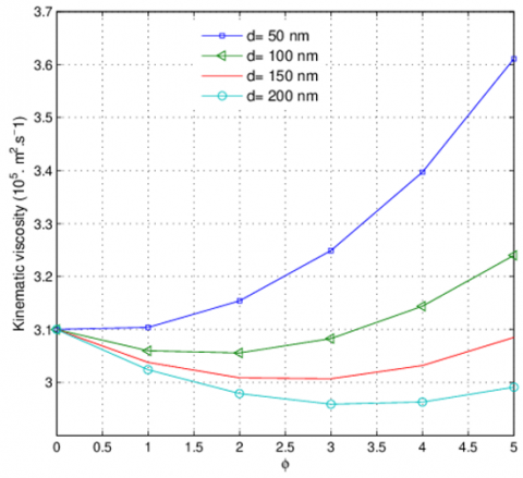
Unlike other models that always predict a decrease in the kinematic viscosity of the nanofluid when volumetric concentration of nanoparticles increases, Figure 2 first predicts a decrease in the kinematic viscosity. Then, an increase from a certain volumetric concentration which depends on the nanoparticles diameter.
Figure 2. Evolution of Kinematic viscosity for WS2-Oil nanofluid with volumetric concentration
2.2 Macroscopic governing equations
The nanofluid flow is assumed incompressible and viscous. The flow is conceived as laminar and two-dimensional. Fluid and solid flow at the same velocity assuming there is no slip between fluid and nanoparticles.
The governing dimensionless equations are as follows:
Continuity equation:
$\frac{\partial U}{\partial X}+\frac{\partial U}{\partial Y}=0$ (3)
Momentum equations:
$\frac{\partial U}{\partial t^{\prime}}+U \cdot \frac{\partial U}{\partial X}+V \cdot \frac{\partial U}{\partial Y}=-\frac{\partial P}{\partial X}+v_d\left(\frac{\partial^2 U}{\partial X^2}+\frac{\partial^2 U}{\partial Y^2}\right)$ (4)
$\frac{\partial V}{\partial t^{\prime}}+U \cdot \frac{\partial V}{\partial X}+V \cdot \frac{\partial V}{\partial Y}=-\frac{\partial P}{\partial Y}+v_d\left(\frac{\partial^2 V}{\partial X^2}+\frac{\partial^2 V}{\partial Y^2}\right)$ (5)
where, $v_d$ is the dimensionless kinematic viscosity given by:
$v_d=\frac{\mu_{n f}}{\mu_{b f}} \frac{\rho_{b f}}{\rho_{n f}} \frac{1}{R_e}=\frac{1}{\left(1-34.87\left(d_p / d_{b f}\right)^{-0.3} \varphi^{1.03}\right)} \cdot \frac{1}{\left((1-\varphi)+\varphi \rho_s / \rho_{b f}\right)} \frac{1}{R_e}$
$R_e$ is the Reynolds number defined by:
$R_e=\frac{U_0 \cdot H}{v_{b f}}$
$X, Y, U, V, P, t^{\prime}$ are the dimensionless parameters defining as:
$X=x / H, Y=y / H, U=u / U_0, V=v / U_0, t^{\prime}=t \cdot U_0 / H$ and $P=p \cdot \rho_{n f} / U_0^2$. Where x and y represent the Cartesian coordinates, u and v are respectively, the horizontal and vertical velocity and p is the pressure.
The considered parameters are the nanoparticles concentration φ, the flow Reynolds number $R_e$ and the nanoparticle diameter d.
The macroscopic boundary conditions are: $u(x, o)=U_0, u(x, H)=U_0$ and $u(0, y)=u(0, L)=0$.
2.3 Friction factor
The local skin friction at bottom surface (x=0) is defined by:
$C_f=\frac{F_d}{\frac{1}{2} \rho_{n f} \cdot U_r^2}$
where, $U_r$ is a reference velocity taken equal to $U_0$ and $F_d$ is the local skin friction drag at the bottom surface expressed as:
$F_d(x)=-\mu_{n f} \frac{\partial u_x}{\partial y}(x, 0)$
The local skin friction value at bottom surface is therefore expressed as:
$C_f(X)=\frac{-2}{R_e} F(\varphi, d) \frac{1}{\left(1-\varphi+\varphi \frac{\rho_s}{\rho_f}\right)} \frac{\partial U_X}{\partial Y}(X, 0)$ (6)
where, $R_e$ is Reynolds number of base fluid $(\varphi=0)$ and $F(\varphi, d)$ is function of $\varphi$ and $d$ defined as:
$F(\varphi, d)=\frac{1}{1-34.87\left(d / d_{b f}\right)^{-0.3} \varphi^{1.03}}$
The local skin friction $C_f$ is therefore a function of the following parameters: Reynolds number $R_e$, volumetric concentration of nanoparticles φ, nanoparticle diameter d and horizontal velocity gradients at the bottom surface.
The value of average friction factor at the bottom surface is calculated as:
$C F=\frac{1}{L} \int_0^L C_f(x) d x$
The friction reduction rate δ is calculated as:
$\delta \%=\left|1-\frac{C F(\varphi)}{C F(\varphi=0)}\right| \times 100$
where, CF(φ=0) and CF(φ) are respectively, the average friction factors of the base fluid and nanofluid flows.
3.1 Lattice Boltzmann method
The lattice Boltzmann method uses a mesoscopic approach for modeling flows. In the context of the Boltzmann equation, we use the particle distribution function f which governs the probability of existence of a large number of particles at a point x and at time t in the mesoscopic system. In lattice Boltzmann method, the fluid flow is described using two processes: The first phase is the streaming where there is a transfer of a group of particles on the lattice link according to the directional velocities by which the velocity space is described. The second phase is collision where particles on the same lattice redistribute and relax into their quasi-equilibrium. The application of lattice Boltzmann method uses two main collision models: The first model, in which all moments have the same relaxation rate, is called single relaxation time (SRT) or model (BGK) (Bhatnagar, Gross and Krook) [18]. It is considered the most popular model because of its simplicity. Despite this, the BGK model presents deficiencies in terms of numerical instability and imprecision in the implementation of boundary conditions [19]. In addition to the difficulties encountered in reaching high Reynolds number flows. The lattice Boltzmann equation model (SRT) is written as:
$f_i\left(x+c_i \Delta t, t+\Delta t\right)-f_i(x, t)=\Omega_i=-\frac{1}{\tau}\left(f_i(x, t)-f_i^{e q}(x, t)\right)$ (7)
where, $f_i$ is the particle distribution function with velocity $c_i$ at lattice node, $f_i^{e q}$ is the equilibrium distribution function, $\Omega_i$ is the discrete collision operator, and $\tau$ is the dimensionless relaxation time.
The second model, called Lattice Boltzmann method with multi- relaxation time (MRT-LBM) introduced in reference [20], is more stable than the BGK because the different relaxation times can be individually adjusted to obtain optimal stability [21].
3.2 Multi-relaxation-time lattice Boltzmann model for flow field
In the numerical implementation of the MRT Lattice Boltzmann model for the flow field, the collision step is operated in the moment space while the streaming step occurs in the velocity space. As in references [21, 22], the MRT-LB equation is expressed as follows:
$f_i(x+c i \Delta t, t+\Delta t)-f_i(x, t)=M^{-1} S\left(m_i(x, t)-m_{e q}\right)$ (8)
where, S is the relaxation matrix and M is the orthogonal transformation matrix constricted from velocity. m and $m_{e q}$ are vectors of moments.
In this work, the $D_2 Q_9$ model is used (Figure 3).
Figure 3. Discrete velocity vectors for $D_2 Q_9$ model
The nine discrete velocities ci {i=1, 2, ..., 9} are given by:
$\boldsymbol{c}_i=\left\{\begin{array}{cc}(0,0) & i=1 \\ {\left[\cos (i-1) \frac{\pi}{2}, \sin (i-1) \frac{\pi}{2}\right] c} & i=2,3,4,5 \\ {{\left[\cos (2 i-9) \frac{\pi}{4}, \sin (2 i-9) \frac{\pi}{4}\right] c \sqrt{2}} \quad i=6,7,8,9}\end{array}\right.$
where the lattice speed $c$ is calculated as $c=\frac{\delta \mathrm{x}}{\delta \mathrm{t}}, \delta x$ and $\delta t$ are respectively, the lattice spacing and time step ( $\delta t=$ $\delta x=1)$.
The collision process will occur in terms of momentum rather than velocity. Therefore, the distribution functions based on velocity must be translated into the space of moments. This transformation is achieved through the matrix M, constructed via the Gram-Schmidt procedure [23]. In $D_2 Q_9$ lattice (two-dimensional nine-velocity), the matrix M can be written as:
$M=\left(\begin{array}{ccccccccc}1 & 1 & 1 & 1 & 1 & 1 & 1 & 1 & 1 \\ -4 & -1 & -1 & -1 & -1 & 2 & 2 & 2 & 2 \\ 4 & -2 & -2 & -2 & -2 & 1 & 1 & 1 & 1 \\ 0 & 1 & 0 & -1 & 0 & 1 & -1 & -1 & 1 \\ 0 & -2 & 0 & 2 & 0 & 1 & -1 & -1 & 1 \\ 0 & 0 & 1 & 0 & -1 & 1 & 1 & -1 & -1 \\ 0 & 0 & -2 & 0 & 2 & 1 & 1 & -1 & -1 \\ 0 & 1 & -1 & 1 & -1 & 0 & 0 & 0 & 0 \\ 0 & 0 & 0 & 0 & 0 & 1 & -1 & 1 & -1\end{array}\right)$
The density distribution function $f_i$ can be projected on to the moment space with $m=f . M$ and $f=M^{-1} . m$.
The nine components of the moment vector m are
$m=\left(m_1, m_2, m_3, m_4, m_5, m_6, m_7, m_8, m_9\right)^T m=\left(\rho, e, \epsilon, j_x, q_x, j_y, q_y, p_{x x}, p_{x y}\right)^T$ (9)
where, $\rho$ is the density, $e$ is related to energy, $\epsilon$ is related to energy square, $j_x=\rho u_x$ and $j_y=\rho u_y$ are respectively the components of the momentum flux components along $x$ and $y$ directions, $q_x$ and $q_y$ correspond to the $x$ and $y$ components of the energy flux, $p_{x x}$ and $p_{x y}$ correspond to the symmetric and traceless components of the strain-rate tensor.
In the spatial transformation of velocity into moment, the only hydrodynamic moments that are locally conserved are the scalar density ρ and the moment $j=\left(j_x, j_y\right)$, since all others are non-conserved kinetics moments.
The equilibrium moments $m_{e q}$ are given by:
$m\left\{\begin{array}{c}m_1^{e q}=\rho \\ m_2^{e q}=e=-2 \rho+3\left(j_x^2+j_y^2\right) \\ m_3^{e q}=\epsilon=\rho-3\left(j_x^2+j_y^2\right) \\ m_4^{e q}=j_x \\ m_5^{e q}=q_x=-j_x \\ m_6^{e q}=j_y \\ m_7^{e q}=q_y=-j_y \\ m_8^{e q}=p_{x x}=\left(j_x^2-j_y^2\right) \\ m_9^{e q}=p_{x y}=j_x \cdot j_y\end{array}\right.$ (10)
The collision matrix S, is a diagonal matrix containing the relaxation coefficients associated with each of the moments. The relaxation matrix has the following form:
$S=\operatorname{diag}\left(s_1, s_2, s_3, s_4, s_5, s_6, s_7, s_8, s_9\right)$
where, the $S_K\{k=1,2, \ldots, 9\}$ are the relaxation parameters determined by a linear stability analysis $[18]\left(S_k \in\right] 0,2[)$. The coefficients $s_8$ and $s_9$ are related to the viscosity in lattice units $v_{L B}$ by the relation:
$s_8=s_9=\frac{2}{1+6 v_{L B}}$
The other coefficients were chosen as follows: $s_1=s_4=$ $s_6=1 ; s_2=s_3=1.4 ; s_5=s_7=1.2$.
From the moments of the distribution functions, the macroscopic fluid quantities, density ρ and velocity $\vec{u}$ are obtained as follows:
$\rho=\sum_{i=1}^9 f_i$ (11)
$\rho \vec{u}=\sum_{i=1}^9 \vec{c}_i \cdot f_i$ (12)
3.3 Boundary conditions
The unknown distribution functions pointing to the fluid zone at the boundaries nodes must be specified. For the right and left fixed vertical walls, a bounce-back boundary is used. After collision, the incoming boundary populations are equal to the out-going populations. For example, for the left boundary, the following conditions are imposed:
$\left\{\begin{array}{l}f_6=f_8 \\ f_2=f_4 \\ f_9=f_7\end{array}\right.$
For the top and bottom moving walls with a given speed, The Zou-He boundary conditions were applied. For example, for the top boundary, unknown density distribution functions can be determined by the following conditions:
$\left\{\begin{array}{c}f_5=f_3 \\ f_8=f_6+\frac{1}{2}\left(f_2-f_4\right)-\frac{1}{2} \rho U_0 \\ f_9=f_7+\frac{1}{2}\left(f_4-f_2\right)+\frac{1}{2} \rho U_0\end{array}\right.$
3.4 Numerical procedure
The procedure for numerical resolution of the lattice Boltzmann equation includes the collision and streaming steps, application of boundary conditions, calculation of particle distribution function and finally calculation of macroscopic variables. The algorithm of resolution is specified as below:
1. Discretization of physical domain and calculation of the simulation parameters.
2. Initialization of distribution functions to their equilibrium value.
3. Collision step:
$f_i(\vec{x}, t+1)=f_i(\vec{x}, t)-\boldsymbol{M}^{-1} \boldsymbol{S}\left[m_i(\vec{x}, t)-m_i^{e q}(\vec{x}, t)\right]$
$(\delta t=\delta x=1)$
4. Application of boundary conditions;
5. Streaming step: $f_i\left(\vec{x}+\overrightarrow{c_l}, t+1\right)=f_i(\vec{x}, t+1)$;
6. Calculation of macroscopic variables (Eq. (11) and Eq. (12));
7. Check the convergence criterion - if convergence reached, then finish the calculations - if not, repeat from 3 where convergence is considered reached if the following criterion is satisfied:
$\frac{\left|\sqrt{\left(u_x^2+u_y^2\right)_{n+1}}-\sqrt{\left(u_x^2+u_y^2\right)_n}\right|}{\sqrt{\left(u_x^2+u_y^2\right)_{n+1}}} \leq 10^{-8}$
4.1 Grid independency study and code validation
A MATLAB code has been developed to run the simulation. To terminate the numerical simulation, a convergence criterion of $10^{-8}$ for velocity has been used. The present code was tested for grid independence by calculating the average friction factor at bottom surface. We choose a regular mesh of size $N_x \times N_y$. Different mesh combinations were explored for the case Re=100 and φ=0. The result given in Table 2 showed difference is less than 1% betwen the studied grid size 401×100 and 441× 110. The grid size 401 ×100 ensures a grid independent solution for the studied case.
Table 2. Grid independence study for Re=100 and φ=0
|
Grid size |
CF |
∆ |
|
241×60 |
0.477985 |
- |
|
321×80 |
0.493287 |
3.2% |
|
401×100 |
0.499276 |
% |
|
441×110 |
0.500043 |
0.15% |
$\Delta=100 \times \frac{C F_{n+1}-C F_n}{C F_n}$
A similar study shows that grid size 441×120 provide a grid independent solution for Re=500.
Figure 4. Horizontal and vertical velocities along their respective centerline of the cavity flow at Re=400
The code performance is tested in the problem of the cavity doubly driven by upper and lower covers in case of opposite movements. It is a square cavity where top and bottom walls are moving with uniform velocity in the opposite direction. In Figure 4, the developed velocity profiles were compared with the results presented in reference [24]. A good agreement is observed as shown in this figure.
4.2 Effect of nanoparticle diameter
The various research works have attributed the exceptional properties of friction reduction by lubrication nanoadditives to intermolecular interactions and in particular to the modification of the viscosity. The local skin friction, being proportional to the viscosity, the average friction factor will practically follow the kinematic viscosity evolution.
Figure 5. Average friction factor with volumetric concentration of nanoparticles (a) Re=100 and (b) Re=500
Figure 5 represents the evolution of the average friction factor as a function of the volumetric concentration of nanoparticles for different diameters. This figure shows that evolution takes place in two phases: First a phase of decrease in CF which will take place for low values of the volumetric concentration. Then, a second phase where the average friction factor CF begins to increase from a certain value of volumetric concentration of nanoparticles which depends on the diameter of the nanoparticles. The figure, also, shows that low values of average friction factor are always obtained for large diameter nanoparticles. To verify their reliability, these results are compared to the experimental results of reference [25] in which the tribological properties of nanoparticles of different sizes were tested. In this tribological test, silica nanoparticles with 100nm diameter performed better than silica nanoparticles with 20nm diameter. It could be concluded from the result of this experience that, with the increase of nanoparticle size, the average coefficient of friction CF decrease.
Figure 6. Average friction factor with nanoparticles diameter at Re=500
In Figure 6, the average friction factor evolutions for two values of the volumetric concentration of nanoparticles (φ=2% and φ=4%) are compared. This figure shows that by increasing the nanoparticles diameter, the average friction coefficient CF decreases and that the values of CF for the volumetric concentration φ=2% are always lower than those obtained for φ=4%. This trend is reversed above a diameter value of around 180nm.
Figure 7 represents the variations of friction reduction rate with the nanoparticles volumetric concentration of nanoparticles for two values of the nanoparticles diameter. The best reduction rate is always obtained with nanoparticles of large diameter = 200nm. The maximum reduction is obtained for volumetric concentration of nanoparticles φ=3%. The maximum reduction rate is $\tau_{\max }$=4%.
Figure 7. Friction reduction rate with volumetric concentration of nanoparticles at Re=500
In the present work, an incompressible D2Q9MRT model is used to simulate the flow of the 5W30 Oil-WS2 nanofluid confined by two moving surfaces. The effects of nanoparticles diameter on friction reduction have been studied. The obtained result has shown that the use of large diameter nanoparticles with a low volumetric fraction leads to the best friction reduction rate. It was found that the predict results agreed well with the published experimental results.
|
Re |
Reynolds number |
|
u,v |
components of velocity (m. $s^{-1}$) |
|
U,V |
dimensionless of velocity component |
|
x,y |
Cartesian coordinates (m) |
|
X,Y |
dimensionless of Cartesian coordinates |
|
p |
pressure($K g . m^{-1} s^{-2}$) |
|
L |
length of the cavity (m) |
|
H |
cavity height (m) |
|
$f_i$ |
density distribution function |
|
$f_i^{e q}$ |
equilibrium distribution function |
|
$c_i$ |
discrete particle velocity |
|
$U_0$ |
uniform velocity of moving plates (m. $s^{-1}$) |
|
$C_f$ |
local skin friction |
|
MRT |
multiple relaxation time |
|
LB |
lattice Boltzmann |
|
CF |
average friction factor |
|
d |
nanoparticle diameter (m) |
|
Greek symbols |
|
|
$\mu_{n f}$ |
dynamic viscosity of nanofluid ($K g . m^{-1} . s^{-1}$) |
|
$\mu_f$ |
dynamic viscosity of base fluid ($K g . m^{-1} . s^{-1}$) |
|
$\rho_{n f}$ |
effective density of nanofluid ($K g . m^{-1} . s^{-1}$) |
|
$\rho_{b f}$ |
base fluid density ($K g . m^{-3}$) |
|
$\rho_s$ |
nanoparticles density ($K g . m^{-3}$) |
|
φ |
nanofluid volumetric concentration |
|
$v_{L B}$ |
viscosity in lattice units |
|
τ |
dimensionless relaxation time |
[1] He, F., Xie, G., Luo, J. (2020). Electrical bearing failures in electric vehicles. Friction, 8(1): 4-28. https://doi.org/10.1007/s40544-019-0356-5
[2] Holmberg, K., Erdemir, A. (2017). Influence of tribology on global energy consumption, costs and emissions. Friction, 5(3): 263-284. https://doi.org/10.1007/s40544-017-0183-5
[3] Bartz, W.J. (1972). Some investigations on the influence of particle size on the lubricating effectiveness of molybdenum disulfide. Asle Transactions, 15(3): 207-215. https://doi.org/10.1080/05698197208981418
[4] Rapoport, L., Lvovsky, M., Lapsker, I., Leshchinsky, V., Volovik, Y., Feldman, Y., Tenne, R. (2001). Slow release of fullerene-like WS2 nanoparticles from Fe- Ni graphite matrix: a self-lubricating nanocomposite. Nano Letters, 1(3): 137-140. https://doi.org/10.1021/nl005516v
[5] Bondarev, A.V., Fraile, A., Polcar, T., Shtansky, D.V. (2020). Mechanisms of friction and wear reduction by h-BN nanosheet and spherical W nanoparticle additives to base oil: Experimental study and molecular dynamics simulation. Tribology International, 151: 6493. ttps://doi.org/10.1016/j.triboint.2020.106493
[6] Azaditalab, M., Houshmand, A., Sedaghat, A. (2016). Numerical study on skin friction reduction of nanofluid flows in a Taylor–Couette system. Tribology International, 94: 329-335. https://doi.org/10.1016/j.triboint.2015.09.046
[7] Hrour, S., Bahraoui, F., Hrour, E. (2020). Numeric study on skin friction reduction of engine Oil-WS2 nanofluid by MRT lattice boltzman method. Journal of Materials Science and Engineering A, 10(7-8): 132-141. https://doi.org/10.17265/2161-6213/2020.7-8.003
[8] Hu, Y., Li, D., Shu, S., Niu, X. (2015). Study of multiple steady solutions for the 2D natural convection in a concentric horizontal annulus with a constant heat flux wall using immersed boundary-lattice Boltzmann method. International Journal of Heat and Mass Transfer, 81: 591-601. https://doi.org/10.1016/j.ijheatmasstransfer.2014.10.050
[9] Nie, X., Doolen, G.D., Chen, S. (2002). Lattice-Boltzmann simulations of fluid flows in MEMS. Journal of statistical physics, 107(1): 279-289. https://doi.org/10.1023/A:1014523007427
[10] Semma, E., El Ganaoui, M., Bennacer, R., Mohamad, A. A. (2008). Investigation of flows in solidification by using the lattice Boltzmann method. International Journal of Thermal Sciences, 47(3): 201-208. https://doi.org/10.1016/j.ijthermalsci.2007.02.010
[11] Hu, Y., Li, D., Shu, S., Niu, X. (2015). Modified momentum exchange method for fluid-particle interactions in the lattice Boltzmann method. Physical Review E, 91(3): 033301. https://doi.org/10.1103/PhysRevE.91.033301
[12] Valizadeh Ardalan, M., Alizadeh, R., Fattahi, A., Adelian Rasi, N., Doranehgard, M.H., Karimi, N. (2021). Analysis of unsteady mixed convection of Cu–water nanofluid in an oscillatory, lid-driven enclosure using lattice Boltzmann method. Journal of Thermal Analysis and Calorimetry, 145(4): 2045-2061. https://doi.org/10.1007/s10973-020-09789-3
[13] Ahrar, A.J., Djavareshkian, M.H. (2016). Lattice Boltzmann simulation of a Cu-water nanofluid filled cavity in order to investigate the influence of volume fraction and magnetic field specifications on flow and heat transfer. Journal of Molecular Liquids, 215: 328-338. https://doi.org/10.1016/j.molliq.2015.11.044
[14] Pak, B.C., Cho, Y.I. (1998). Hydrodynamic and heat transfer study of dispersed fluids with submicron metallic oxide particles. Experimental Heat Transfer an International Journal, 11(2): 151-170. https://doi.org/10.1080/08916159808946559
[15] Einstein, A. (1905). Eine neue bestimmung der moleküldimensionen. Doctoral dissertation, ETH Zurich.
[16] Brinkman, H.C. (1952). The viscosity of concentrated suspensions and solutions. The Journal of chemical physics, 20(4): 571-571. https://doi.org/10.1063/1.1700493
[17] Corcione, M. (2011). Empirical correlating equations for predicting the effective thermal conductivity and dynamic viscosity of nanofluids. Energy conversion and management, 52(1): 789-793. https://doi.org/10.1016/j.enconman.2010.06.072
[18] Bhatnagar, P.L., Gross, E.P., Krook, M. (1954). A model for collision processes in gases. I. small amplitude processes in charged and neutral one-component systems. Phys. Rev., 94: 511. https://doi.org/10.1103/PhysRev.94.511
[19] Ginzburg, I., d’Humières, D. (2003). Multireflection boundary conditions for lattice Boltzmann models. Phys Rev. E., 68: 066614. https://doi.org/10.1103/PhysRevE.68.066614
[20] d’Humières, D. (1992). Generalized lattice-Boltzmann equations. Theory and Simulations, 159: 450-458. https://doi.org/10.2514/5.9781600866319.0450.0458
[21] Lallemand, P., Luo, L.S. (2000). Theory of the lattice Boltzmann method: Dispersion, dissipation, isotropy, Galilean invariance, and stability. Physical Review E, 61(6): 6546. https://doi.org/10.1103/PhysRevE.61.6546I.
[22] Lallemand, P., Luo, L.S. (2003). Theory of the lattice Boltzmann method: Acoustic and thermal properties in two and three dimensions. Physical review E, 68(3): 036706. https://doi.org/10.1103/PhysRevE.68.036706
[23] Bouzidi, M., DHumieres, D., Lallemand, P., Luo, L.S., Bushnell, D.M. (2002). Lattice Boltzmann equation on a 2D rectangular grid (No. NASA/CR-2002-211658).
[24] Perumal, D.A., Dass, A.K. (2008). Simulation of flow in two-sided lid-driven square cavities by the lattice Boltzmann method. WIT Transactions on Engineering Sciences, 59: 45-54. https://doi.org/10.2495/AFM080051
[25] Sui, T., Song, B., Zhang, F., Yang, Q. (2015). Effect of particle size and ligand on the tribological properties of amino functionalized hairy silica nanoparticles as an additive to polyalphaolefin. Journal of Nanomaterials, 16: 427. https://doi.org/10.1155/2015/492401