Ariful Islam* | Badhan Das | Lasker Ershad Ali | Md. Azizur Rahman
© 2022 IIETA. This article is published by IIETA and is licensed under the CC BY 4.0 license (http://creativecommons.org/licenses/by/4.0/).
OPEN ACCESS
A computational analysis on transient magnetohydrodynamics micropolar fluid flow through a non-Darcy porous medium has been investigated. A computer code based on finite difference technique was developed in Fortran programming language with the objective to analyze the behavior of fluid flow in a porous medium for the non-Darcy case. Two-dimensional mathematical model of the problem has been utilized to obtain the non-similar solutions. The finite difference technique was used to explicitly solve the dimensionless equations of fluid velocity, temperature, angular velocity, and concentration to study the behavior of the system for various parameters. In addition, the stability of the system has been performed and obtained that the system converged for the values of Prandtl and Schmidt number greater than and equal to 0.03. The behavior of the system was studied for non-dimensional time ranging from 0 to 80 for a small-time step of 0.005. The most significant influence of various parameters on fluid velocity, temperature, angular velocity, and concentration profiles within the boundary layer have represented graphically and discussed qualitatively. It was found that the system reached to a steady state at the time greater than or equal to 75.
micropolar fluid, non-Darcy porous medium, magnetic field
The micropolar fluid flow behavior has a significant impact in the research areas of industrial processes such as polymer sheet extrusion, plastic film drawing, growing crystal, hot rolling, paper and glass fiber production, metal spinning, and so on [1-4]. It is common that the micropolar fluid flow is affected by the shear behavior of fluid. In fact, it is still difficult to examine the shear behavior of fluid for the cases of Newtonian relationship. A new principle in the assessment of fluid dynamics theory is still under development. More importantly, the analysis of the micropolar fluid behavior for the case of a non-Darcy porous medium is scarce in the published literature.
Micropolar fluid theory was invented by Eringen [5], who considered micro-rotational motion and inertial effects on fluid that display couple stress and distributed body moments. They noted that the spin inertia has a direct consequence on stress and body moments. Gorla [6] studied numericaly the boundary layer solutions for the flow of micropolar fluid in both forced and free convection over a vertical flat plate. Later on Gorla [7] extended the work and found that micropolar fluids have a lower surface heat transfer rate and demonstrated the drug reduction as compared to Newtonian fluids. In the presesence of a magnetic field, viscous Joule heating effect of an MHD micropolar fluid flow has been performed by Abd El-Hakiem et al. [8]. In light of thermal radiation, the suction and injection effects of a micropolar fluid flow through a constantly moving plate was analyzed by El-Arabawy [9]. It has been demonstrated that for increasing the value of suction and thermal parameter the heat transfer rate increased monotonically. In addition, for decreasing values of the injection parameter the rate of heat transfer decreased.
On the other hand, Ganesan and Palani [10] solved the magnetohydrodynamic unsteady fluid flow model along an inclined plate by using implicit finite difference technique. They found that the concentration profile decreased with increasing values of Schmidt number. In addition, Abo-Eldahab and Ghonaim [11] studied the radiation effect on micropolar fluid that flows along a stationary porous plate. It has been noted that the angular velocity increased due to the boost of vortex-viscosity parameter. Over a vertical porous plate, Islam et al. [12] investigated the flow behavior of micropolar fluid in the presence of magnetic field by using the finite difference technique. They studied the fluid flow behavior for different values of microrotation parameter. It can be observed from their illustrated numerical values that the fluid velocity increased with microrotation parameter.
Furthermore, Palani and Kim [13] numerically analyzed the viscous dissipation and Joule heating effect on MHD free convection flow considering a variable surface temperature. They discovered that the Lorentz force, a resistive form of force, which slows down fluid velocity, is caused by the transverse magnetic field. Homotopic incompressible micropolar biofluid flow between two parallel porous plates in the presence of magnetic field has been executed by Bég et al. [14]. They observed that the growing effects of spin gradient viscosity leads to increase in the angular velocity.
For the case of MHD free convection micropolar fluid flow along a vertical porous plate it was found that the angular fluid motion was higher for lighter particles than the heavier particles [15]. In addition, the microrotation of micropolar fluid was observed to be decreased to zero for increasing values of spin gradient viscosity parameter in the presence of magnetic field [16]. Moreover, casson fluid flow through an unsteady stretched surface with chemical reaction and convective boundary conditions has been depicted by Thammanna et al. [17]. It can be seen from their plotted results that the larger values of casson parameter decreased the velocity components. The Prandtl number has also been shown to have a negative effect on the thermal boundary layer thickness. Bég et al. [18] executed an investigation of MHD heat generation mass transfer flow of a fluid that passed through an inclined plate with Soret effects. It has been noted that the magnetic field droops the boundary layer flow. In 2021, Haque [19] investigated the effect of induced magnetic field on a micropolar fluid flow through a semi-infinite plate. He noted that the steady state solution arises when the induced magnetic field and microrotation increased. However, the study of micropolar fluid flow in the presence of non-Darcy porous media has not been adequately considered [19].
It is important to add a non-Darcy behavior into the system when dealing with high fluid velocity to investigate the MHD free convection flow of micropolar fluid. The Forchheimer number can be used to interpret non-Darcy flow in the porous media by adding a second order velocity term to the Darcy equation [20]. Considering a non-Darcy porous system, Pal and Chatterjee [21] investigated the radiation impacts on MHD mixed convection micropolar fluid flow. They observed that the temperature gradient reduces due to the increasing values of Prandtl number. Taking a non-Darcy porous system, the effects of thermal radiation and thermal dispersion of a fluid have been studied by Mohammadien and El-Amin [22]. They discovered that the rate of heat transfer increases with the increase of thermal radiation. In addition, Murthy and Singh [23] investigated the free convection lateral mass flux effect of a fluid that saturated in a non-Darcy porous media.
On natural convection, El-Amin [24] explored the combined effect of a fluid’s thermal and solutal dispersion in a non-Darcy vertical porous plate. In his study, the heat and mass transfer were examined using the Forchheimer flow model in Darcy and non-Darcy cases. Noghrehabadi et al. [25] investigated the steady flow of nanofluids through a non-Darcy porous medium in an isothermal vertical cone on natural convection. It was found that raising the value of the non-Darcy parameter, the temperature and concentration profiles were increased whereas decreased the velocity profile [25]. The influence of chemical reactions and thermal radiation of a MHD non-Newtonian nanofluid that passed through a horizontal non-Darcy stretched sheet have been examined by El-Dabe et al. [26]. They studied the influence of the Forchheimer number, Eckert number, non-Newtonian, and radiation parameters etc. on the stream function, temperature, concentration distributions and nanoparticle volume fraction. In addition, Seth et al. [27] have analyzed the effect of Joule heating, viscous dissipation, and thermo-diffusion on the unsteady flow of Casson fluid along a non-Darcy oscillating porous plate. However, the unsteady magnetohydrodynamic flow of micropolar fluid in a non-Darcy porous medium still scarce in the available published literature.
Considering the research gap, this study explores the unsteady MHD micropolar fluid behavior in a non-Darcy porous medium in which the Forchheimer number has been incorporated in the mathematical model to simulate the system involving a high fluid velocity. Similarity technique is adopted to convert the boundary layer equations into nondimensional form which are explicitly solved by finite difference method. Numerical simulations of the fluid flow related to angular momentum, momentum with others are attained as a functions of the boundary layer. All the solutions of this study are focused on the effect of various parameters including microrotation in non-Darcy porous medium which are discussed and illustrated graphically through a set of figures.
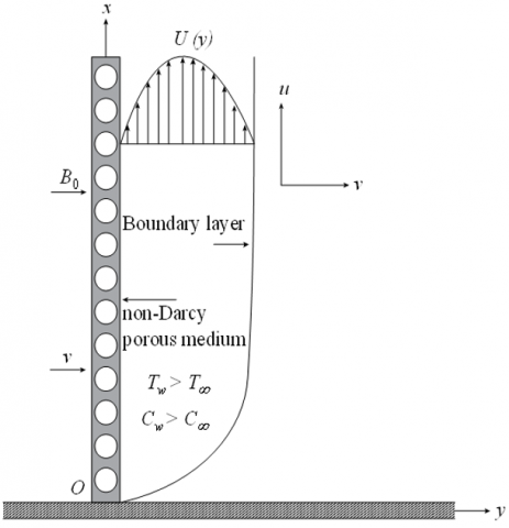
Figure 1 shows the MHD unsteady micropolar fluid flow along the x axis, which is taken along the plate and the y axis is measured normal to the plate. The fluid and plate are first assumed to be at rest, and then the entire system is allowed to revolve with a constant angular momentum component $\Gamma$ around the z axis. Since the system rotates about z axis, so the angular momentum can be assumed as $G=(0,0, \Gamma)$. The temperature of the plate is gradually raised from $T_w$ to $T_{\infty}$, and the concentration $C_w$ to $C_{\infty}$, which are thereafter maintained constant, where $T_w$, $T_{\infty}$ are the uniform fluid temperatures at the wall and beyond the boundary wall, respectively. In addition, $C_w$ and $C_{\infty}$ are the concentrations at the wall and beyond the wall, respectively. Uniform magnetic field $B_0$ is applied perpendicularly to the plate, which is along the boundary layer thickness. Therefore, the coordinate of the magnetic field vector $B=\left(0, B_0, 0\right)$ (Figure 1).
Figure 1. Physical configuration of the model
The mathematical model based on the free convection MHD micropolar fluid flow in a non-Darchy porous medium for the case of a two-dimensional unsteady flow can be considered according to the Eqns. (1)-(5) below:
$\frac{\partial u}{\partial x}+\frac{\partial v}{\partial y}=0$ (1)
$\frac{\partial u}{\partial t}+u \frac{\partial u}{\partial x}+v \frac{\partial u}{\partial y}=g \beta\left(T-T_{\infty}\right)+g \beta^*\left(C-C_{\infty}\right)+$
$\left(v+\frac{\chi}{\rho}\right)\left(\frac{\partial^2 u}{\partial y^2}\right)+\frac{\chi}{\rho} \frac{\partial \Gamma}{\partial y}-\frac{\sigma^{\prime} u B_0^2}{\rho}-\frac{v}{K} u-\frac{c_b}{\sqrt{K}} u^2$ (2)
$\frac{\partial \Gamma}{\partial t}+u \frac{\partial \Gamma}{\partial x}+v \frac{\partial \Gamma}{\partial y}=\frac{\gamma}{\rho j}\left(\frac{\partial^2 \Gamma}{\partial y^2}\right)-\frac{\chi}{\rho j}\left(\frac{\partial u}{\partial y}\right)$ (3)
$\frac{\partial T}{\partial t}+u \frac{\partial T}{\partial x}+v \frac{\partial T}{\partial y}=\frac{k}{\rho c_p} \frac{\partial^2 T}{\partial y^2}+\frac{D_m k_T}{c_p c_s}\left(\frac{\partial^2 C}{\partial y^2}\right)+\frac{v}{c_p}\left(\frac{\partial u}{\partial y}\right)^2$ (4)
$\frac{\partial C}{\partial t}+u \frac{\partial C}{\partial x}+v \frac{\partial C}{\partial y}=D_m \frac{\partial^2 C}{\partial y^2}+\frac{D_m k_T}{c_p c_s}\left(\frac{\partial^2 T}{\partial y^2}\right)$ (5)
The boundary conditions for the above mentioned problem are considered for the time equal to zero and greater than zero. Therefore, the boundary conditions when the time t = 0 can be given by the Eq. (6) below:
$u=0, v=0, C=0, T=0, \Gamma=0$ (6)
For the time t > 0, the boundary conditions can be given by the Eq. (7) below:
$\left.\begin{array}{l}u=0, v=0, C=0, T=0, \Gamma=0, \text { when } x=0 \\ u=0, v=0, C=C_w, T=T_w, \Gamma=1 \text {, when } y=0 \\ u=0, v=0, C=0, T=0, \Gamma=0, \text { when } y \rightarrow \infty\end{array}\right\}$ (7)
where, u, v represents the components of velocity in two dimensional Cartesian co-ordinate system along x and y directions, respectively, $\rho$ is the density of fluid, v is the kinematic viscosity of the fluid, $\chi$ represents the vortex viscosity, K is denoted as the permeability of the porous medium, cb be the constant Forchheimer, σʹ is denoted as the fluid electric conductivity, β is the coefficient of volume expansion, g is the gravitational acceleration, and β*is the coefficient of concentration expansion, γ denotes the spin gradient viscosity, j represents the microinertia per unit mass, k is the thermal conductivity of the medium, cp denotes the specific heat at constant pressure, kT is the thermal diffusion ratio, cs is the concentration susceptibility and Dm represents the coefficient of mass diffusivity.
Now, for solving the equations with the help of finite difference scheme, the following dimensionless quantities have been introduced to convert the governing Eqns. (1) – (5) dimensionless with the help of boundary conditions (6) and (7):
$X=x U_0 / v, Y=y U_0 / v, U=u / U_0, V=v / U_0, \tau=$
$t U_0^2 / v, \Gamma=\bar{\Gamma} U_0^2 / v, \bar{T}=\left(T-T_{\infty}\right) /\left(T_w-T_{\infty}\right), \bar{C}=$
$\left(C-C_{\infty}\right) /\left(C_w-C_{\infty}\right)$
Obtained dimensionless equations are given in Eqns. (8) to (12) below:
$\frac{\partial U}{\partial X}+\frac{\partial V}{\partial Y}=0$ (8)
$\frac{\partial U}{\partial \tau}+U \frac{\partial U}{\partial X}+V \frac{\partial U}{\partial Y}=G_r \bar{T}+G_m \bar{C}+(1+\Delta) \frac{\partial^2 U}{\partial Y^2}+\Delta \frac{\partial \bar{\Gamma}}{\partial Y}-\left(M+\frac{1}{D_a}\right) U-\frac{F_o}{D_a} U^2$ (9)
$\frac{\partial \bar{\Gamma}}{\partial \tau}+U \frac{\partial \bar{\Gamma}}{\partial X}+V \frac{\partial \bar{\Gamma}}{\partial Y}=\Lambda \frac{\partial^2 \bar{\Gamma}}{\partial Y^2}-\lambda \frac{\partial U}{\partial Y}$ (10)
$\frac{\partial \bar{T}}{\partial \tau}+U \frac{\partial \bar{T}}{\partial X}+V \frac{\partial \bar{T}}{\partial Y}=\frac{1}{P_r} \frac{\partial^2 \bar{T}}{\partial Y^2}+D_f \frac{\partial^2 \bar{C}}{\partial Y^2}+E_c\left(\frac{\partial U}{\partial Y}\right)^2$ (11)
$\frac{\partial \bar{C}}{\partial \tau}+U \frac{\partial \bar{C}}{\partial X}+V \frac{\partial \bar{C}}{\partial Y}=\frac{1}{S_c} \frac{\partial^2 \bar{C}}{\partial Y^2}+S_o \frac{\partial^2 \bar{T}}{\partial Y^2}$ (12)
The boundary conditions for the above dimensionless equations for corresponding dimensionless time $\tau=0$ reduced to the form of Eq. (13) below:
$U=0, V=0, \bar{C}=0, \bar{T}=0, \bar{\Gamma}=0$ (13)
In addition, for the dimensionless time $\tau$> 0, the boundary conditions can be given by the Eq. (14) below:
$\left.\begin{array}{l}U=0, V=0, \bar{C}=0, \bar{T}=0, \bar{\Gamma}=0, \text { when } X=0 \\ U=0, V=0, \bar{C}=1, \bar{T}=1, \bar{\Gamma}=1, \text { when } Y=0 \\ U=0, V=0, \bar{C}=0, \bar{T}=0, \bar{\Gamma}=0, \text { when } y \rightarrow \infty\end{array}\right\}$ (14)
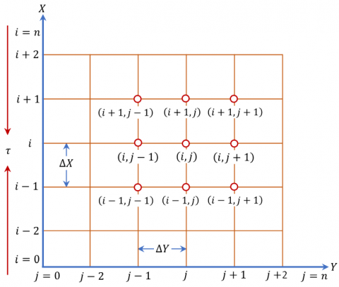
In this section, the governing nonlinear dimensionless partial differential equations have been numerically solved explicitly with the help of associated initial and boundary conditions. Inspired by the work of Callahan and Marner [28]; Soundalgekar and Ganesan [29], this explicit finite difference technique is utilized to analyze the behavior of this current problem. According to the preceding description, the Eqns. (8)-(12) have been solved using the explicit finite difference method along with the boundary conditions (13) and (14). The flow area is split into a grid of mesh for the derivation of governing equations which is shown in Figure 2. The gridlines along the X-axis are parallel to the plate whereas the gridlines along Y-axis are normal to the plate.
Figure 2. Schematic diagram of finite difference grid system
The height and width of the porous plate have been assumed as $X_{\max }$ and $Y_{\max }$, respectively, as $Y \rightarrow \infty$. The X-axis ranges from 0 to 100 whereas, Y -axis ranges from 0 to 70. The grid spacing have been considered as m=125 along X-axis and n = 125 along Y-axis. The mesh sizes are assumed as $\Delta$X = 0.8 and $\Delta$Y = 0.56 along the X and Y axes, respectively, whereas, the time step, $\Delta \tau$ is equal to 0.005. The values of U,V and Γ have been denoted by $U^{\prime}, V^{\prime}$ and $\Gamma^{\prime}$, respectively, at the end of each time step. Therefore, the dimensionless form of the Eqns. (8)-(12) can be given by the Eqns. (15)-(19) below:
$\frac{U_{i, j}-U_{i-1, j}}{\Delta X}+\frac{V_{i, j}-V_{i, j-1}}{\Delta Y}=0$ (15)
$\frac{U_{i, j}^{\prime}-U_{i, j}}{\Delta \tau}+U_{i, j} \frac{U_{i, j}-U_{i-1, j}}{\Delta X}+V_{i, j} \frac{U_{i, j+1}-U_{i, j}}{\Delta Y}=G_r \bar{T}_{i, j}+$
$G_m C_{i, j}+(1+\Delta) \frac{U_{i, j+1}-2 U_{i, j}+U_{i, j-1}}{(\Delta Y)^2}+\Delta \frac{\bar{\Gamma}_{i, j+1}-\bar{\Gamma}_{i, j}}{\Delta Y}-$
$\left(M+\frac{1}{D_a}\right) U_{i, j}-\frac{F_o}{D_a} U_{i, j}^2$ (16)
$\frac{\bar{\Gamma}_{i, j}^{\prime}-\bar{\Gamma}_{i, j}}{\Delta \tau}+U_{i, j} \frac{\bar{\Gamma}_{i, j}-\bar{\Gamma}_{i-1, j}}{\Delta X}+V_{i, j} \frac{\bar{\Gamma}_{i, j+1}-\bar{\Gamma}_{i, j}}{\Delta Y}=$
$\Lambda \frac{\bar{\Gamma}_{i, j+1}-2 \bar{\Gamma}_{i, j}+\bar{\Gamma}_{i, j-1}}{(\Delta Y)^2}-\lambda \frac{U_{i, j+1}-U_{i, j}}{\Delta Y}$ (17)
$\frac{\bar{T}_{i, j}^{\prime}-\bar{T}_{i, j}}{\Delta \tau}+U_{i, j} \frac{\bar{T}_{i, j}-\bar{T}_{i-1, j}}{\Delta X}+V_{i, j} \frac{\bar{T}_{i, j+1}-\bar{T}_{i, j}}{\Delta Y}=$
$\frac{1}{P_r} \frac{\bar{T}_{i, j+1}-2 \bar{T}_{i, j}+\bar{T}_{i, j-1}}{(\Delta Y)^2}+D_f \frac{\bar{C}_{i, j+1}-2 \bar{C}_{i, j}+\bar{C}_{i, j-1}}{(\Delta Y)^2}+$
$E_c\left(\frac{U_{i, j+1}-U_{i, j}}{\Delta Y}\right)^2$ (18)
$\frac{\bar{c}_{i, j}^{\prime}-\bar{c}_{i, j}}{\Delta \tau}+U_{i, j} \frac{\bar{c}_{i, j}-\bar{C}_{i-1, j}}{\Delta X}+V_{i, j} \frac{\bar{c}_{i, j+1}-\bar{C}_{i, j}}{\Delta Y}=$
$\frac{1}{S_C} \frac{\bar{C}_{i, j+1}-2 \bar{C}_{i, j}+\bar{C}_{i, j-1}}{(\Delta Y)^2}+S_o \frac{\bar{T}_{i, j+1}-2 \bar{T}_{i, j}+\bar{T}_{i, j-1}}{(\Delta Y)^2}$ (19)
the corresponding initial and boundary conditions for the above obtained difference equations for time $\tau$ = 0 can be given by the Eq. (20) below:
$U_{i, j}^0=0, V_{i, j}^0=0, \bar{C}_{i, j}^0=0, \bar{T}_{i, j}^0=0, \bar{\Gamma}_{i, j}^0=0$ (20)
Also, for t>0,
$\left.\begin{array}{l}U_{0, j}^n=0, V_{0, j}^n=0, \bar{C}_{0, j}^n=0, \bar{T}_{0, j}^n=0, \Gamma_{0, j}^n=0 \\ U_{i, 0}^n=0, V_{i, 0}^n=0, \bar{C}_{i, 0}^n=1, \bar{T}_{i, 0}^n=1, \Gamma_{i, 0}^n=1 \\ U_{i, L}^n=0, V_{i, L}^n=0, \bar{C}_{i, L}^n=0, \bar{T}_{i, L}^n=0, \Gamma_{i, L}^n=0\end{array}\right\}$ (21)
where, L is tend to infinity.
The mesh points along the x and y axes are designated by the subscripts i and j, respectively. The value of time $\tau$ is equal to $n \Delta \tau$ is denoted by the superscript n, where n=0, 1, 2, 3 ... The values of $U, \bar{\Gamma}, \bar{T}$ and $\bar{C}$ are known considering to the initial conditions (20), at $\tau=0$. The coefficients of $U_{i, j}$ and $V_{i, j}$ in Eqns. (15) to (19) have been determined as constant for every iteration. Using the finite difference approximation technique, the new velocity profile, temperature distribution, concentration and microrotation are at the interior nodal points $U^{\prime}$, $\bar{T}^{\prime}$, $\bar{C}^{\prime}$, and, $\bar{\Gamma}^{\prime}$ respectively. According to the stability analysis, the system of difference equations is coverged for the following criterion:
$U \frac{\Delta \tau}{\Delta X}+|V| \frac{\Delta \tau}{\Delta Y}+\frac{2}{P_r} \frac{\Delta \tau}{(\Delta Y)^2} \leq 1$ and $U \frac{\Delta \tau}{\Delta X}+|V| \frac{\Delta \tau}{\Delta Y}+\frac{2}{S_c} \frac{\Delta \tau}{(\Delta Y)^2} \leq 1$
Due to brevity the stability and convergence analysis are not shown in details here. Since from the initial condition, U=V=0 at τ=0, and for the values Δτ=0.005, ΔX=0.8, ΔY=0.56 the above noted criterion provide $P_r \geq 0.03$ and $S_c \geq 0.03$ respectively.
In this model, a note on transient magnetohydrodynamic free convection micropolar fluid flow over a non-Darcy porous plate has been illustrated. To investigate the behaviour of the system, the finite difference method was used to compute the numerical values of fluid velocity, temperature, microrotation and concentration. The numerical values of fluid flow were obtained for different values of Grashof number (Gr), Darcy number (Da), Modified Grashof number (Gm), Forchheimer number (Fo), Prandtl number (Pr), Spin gradient viscosity parameter (L), Magnetic parameter (M), Microrotational parameter (D), Dufour number (Df), Vortex viscosity parameter (l), Schmidt number (Sc), Eckert number (Ec) and Soret number (So). The main objective of this study was to analyze the flow behavior from the beginning of the simulation to the steady state for different values of the parameters noted above. The simulation results suggest a little changes of flow pattern at time $\tau$ = 20, 60, 70. However, when the time reached to the value 75, the results remain essentially the same. Thus, the steady state conditions have been obtained at time greater than or equal to 75. The steady state solutions as well as the effects of various parameters are depicted in the Figures 3-10 for the time ranging from 20 to 80.
5.1 Effects of Grashof number on fluid velocity
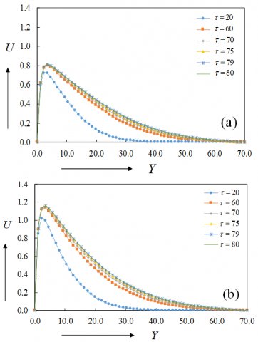
Figure 3. Fluid velocity as a function of Y (boundary layer thickness) for different times when the value of Grashof number (Gr) equal to (a) 0.2 and (b) 0.8. The values of Gm, $\Delta$, M, Da, Fo, $\Lambda, \lambda$, Pr, Df, Ec, Sc and So were equal to 1.0, 0.1, 0.2, 1.0, 0.1, 0.5, 0.1, 0.71, 0.5, 0.1, 0.22 and 0.6, respectively
Figures 3a and b show the fluid velocity for different times from $\tau$ = 20 to 80 for a value of Grashof number (Gr) equal to 0.2 and 0.8, respectively. The values of Gm, $\Delta$, M, Da, Fo, $\Lambda, \lambda$, Pr, Df, Ec, Sc and So are constant and equal to 1.0, 0.1, 0.2, 1.0, 0.1, 0.5, 0.1, 0.71, 0.5, 0.1, 0.22, 0.6, respectively. The velocity increases at the beginning of the simulation process and reaches to zero at the end of the process with the value of Y increases for both the values of Grashof number (Figures 3a and b). In addition, the flow pattern is higher at time $\tau$ = 80 than at $\tau$ = 20. Furthermore, it has been observed that the fluid velocity reached to a steady state value for the time greater than or equal to 75 (Figures 3a and b). It is important to note that the fluid velocity is higher for a larger value of Gr (Figure 3b) than to a lower value (Figure 3a). However, for both cases, the steady state solution is obtained for the time greater than or equal to 75 (Figures 3a and b).
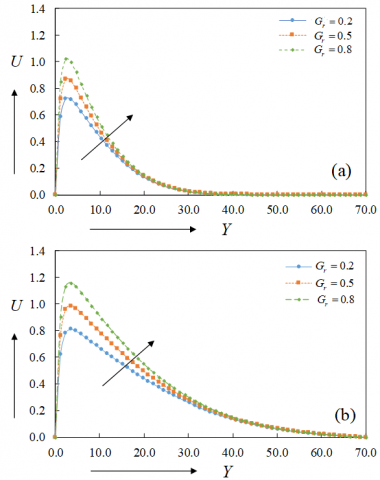
Figure 4. Fluid velocity as a function of Y for different values of Grashof number (Gr) at times (a) $\tau$ = 20 and (b) $\tau$ = 80. The values of Gm, $\Delta$, M, Da, Fo, $\Lambda, \lambda$, Pr, Df, Ec, Scand So equal to 1.0, 0.1, 0.2, 1.0, 0.1, 0.5, 0.1, 0.71, 0.5, 0.1, 0.22 and 0.6, respectively
Figures 4a and b illustrate the fluid velocity for various values of Grashof number (Gr = 0.2, 0.5, 0.8) for the time $\tau$ equal to 20 and 80, respectively. It has been observed that for increasing values of Grashof number the velocity profile increased for both cases. In addition, the fluid velocity was higher at time $\tau$ equal to 80 than at time $\tau$ equal to 20. In contrast, the velocity profiles reached to zero for increasing values of boundary layer thickness (Figures 4a and b). Furthermore, it is important to note that at time $\tau$ equal to 20 the velocity profiles approached to zero when the value of Y is greater than or equal to 30 (Figure 4a). On the other hand, at time $\tau$ equal to 80 the velocity profiles approached to zero when the value of Y is greater than or equal to 60 (Figure 4b). This result is consistent with the published works of Ali et al. [16]. The magnetohydrodynamic micropolar fluid behaviour in the absence of non-Darchy porous medium was studied by using finite difference method [16]. They had obtained that for increasing values of Grashof number the flow velocity increased.
However, the velocity was higher for the case of Ali et al. [16] than the current study of this paper. For a value of Grachoff number equal to 0.2, the flow velocity was equal to 1.25 at time 80 for the case of Ali et al. [16]. However, for a similar value of Grachoff number (0.2), the flow velocity was 0.8 at time 80 for the present study of this paper. It could be the effect of non-Darcy flow in porous medium for MHD micropolar fluid. Most importantly, these two systems are different, therefore, a direct comparison isn’t straight forward.
5.2 Effects of magnetic parameter on fluid velocity
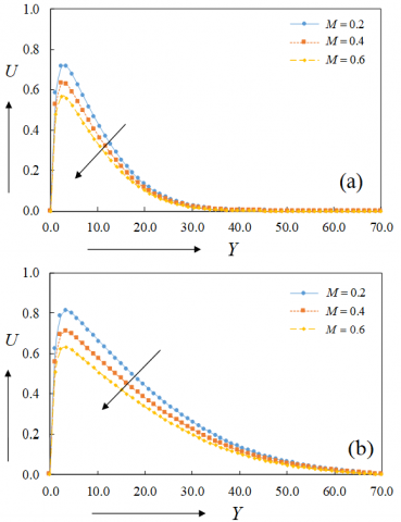
The effect of different values of Magnetic parameter (M = 0.2, 0.4, 0.6) have been depicted at time $\tau$ equal to 20 and 80 in Figures 5a and b, respectively. In both circumstances we can see that for raising the value of magnetic parameter caused the velocity profile to drop. This could be the effect of magnetic parameter, which corresponds to a higher Lorentzian magnetohydrodynamic drag force that works in the opposite direction of the applied magnetic field. This magnetic field obstructing boundary layer flow and resulting in an increase in momentum boundary layer thickness [13, 18]. In addition, for the case of time $\tau$ equal to 20 and 80, the velocity profiles reached to zero when Y was greater than or equal to 30 (Figure 5a) and 60 (Figure 5b), respectively. Furthermore, the fluid velocity was observed to be higher at the beginning (Figure 5a, $\tau$ = 20) than at the steady state (Figure 5b, $\tau$ = 80) of the simulation process.
Figure 5. Fluid velocity as a function of Y for different values of Magnetic parameter (M) at times (a) $\tau$ = 20 and (b) $\tau$ = 80. The values of Gr, Gm, $\Delta$, Da, Fo, $\Lambda, \lambda$, Pr, Df, Ec, Scand So equal to 0.2, 1.0, 0.1, 1.0, 0.1, 0.5, 0.1, 0.71, 0.5, 0.1, 0.22 and 0.6, respectively
5.3 Effects of Forchheimer number on fluid velocity
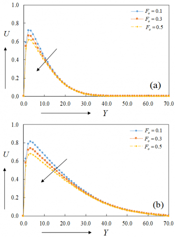
The effect of Forchheimer number on fluid velocity has been investigated and presented on Figures 6a and b at time $\tau$ = 20 and 80, respectively. The values of Forchheimer number ranged from 0.1 to 0.5. The numerical results demonstrated that the velocity profile reduced when the Forchheimer number increased. This phenomenon regarding fluid velocity for different values of Forchheimer number is consistent with the published works of El-Amin [24]. He studied the flow behaviour for both the Darcy and non-Darcy cases. It had been found that for increasing values of Forchheimer number the velocity profile decreased. However, the velocity pattern is different as these two systems (El-Amin [24] and current study of this paper) are not completely identical. In addition, for the case of time $\tau$ equal to 20 and 80, the velocity profiles reached to zero when Y is greater than or equal to 30 (Figure 6a) and 70 (Figure 6b), respectively. Furthermore, the velocity profile was observed to be higher at the beginning (Figure 6a, $\tau$ = 20) than at the steady state (Figure 6b, $\tau$ = 80).
Figure 6. Fluid velocity as a function of Y for different values of Forchheimer number (Fo) at times (a) $\tau$ = 20 and (b) $\tau$ = 80. The values of Gr, Gm, $\Delta$, M, Da, $\Lambda, \lambda$, Pr, Df, Ec, Sc and So are equal to 0.2, 1.0, 0.1, 0.2, 1.0, 0.5, 0.1, 0.71, 0.5, 0.1, 0.22 and 0.6, respectively
5.4 Effects of spin gradient viscosity parameter on fluid angular velocity
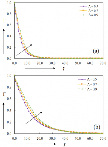
Figures 7a and b show the impact of L (spin gradient viscosity parameter) on the angular velocity profile at time $\tau$ = 20 and 80, respectively. The values of L ranging from 0.5 to 0.9. It has been observed that for increasing values of microrotational parameter, the angular velocity increased. This increasing in angular velocity distribution is consistent with the published paper of Bég et al. [14]. In addition, for the case of time $\tau$ = 20 and 80, the angular velocity profiles reached to zero when Y is greater than or equal to 30 (Figure 7a) and 60 (Figure 7b), respectively. Furthermore, the angular velocity profiles were observed to be higher at the beginning (Figure 7a, $\tau$ = 20) than at the steady state (Figure 7b, $\tau$ = 80).
Figure 7. Fluid angular velocity as a function of Y for different values of L at times (a) $\tau$ = 20 and (b) $\tau$ = 80. The values of Gr, Gm, $\Delta$, M, Da, Fo, l, Pr, Df, Ec, Sc and So are equal to 0.2, 1.0, 0.1, 0.2, 1.0, 0.1, 0.1, 0.71, 0.5, 0.1, 0.22 and 0.6, respectively
5.5 Effects of vortex viscosity parameter on fluid angular velocity
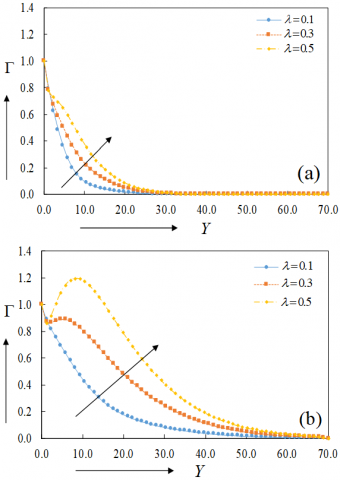
The influence of different values of the vortex viscosity parameter (l = 0.1, 0.3, 0.5) has been explored in Figures 8a and b at time t=20 and 80, respectively. It has been discovered that for increasing values of the vortex viscosity parameter the angular velocity increased. In addition, for the case of time $\tau$ = 20 and 80, the angular velocity profiles reached to zero when Y is greater than or equal to 30 (Figure 8a) and 60 (Figure 8b), respectively. Furthermore, a sudden increase in the angular velocity was observed for a vortex viscosity parameter of 0.5 at time t=80 (Figure 8b), which requires a further investigation.
Figure 8. Fluid angular velocity as a function of Y for different values of vortex viscosity parameter (l) at times (a) $\tau$ = 20 and (b) $\tau$ = 80. The values of Gr, Gm, $\Delta$, M, Da, Fo, L, Pr, Df, Ec, Sc and So are equal to 0.2, 1.0, 0.1, 0.2, 1.0, 0.1, 0.5, 0.71, 0.5, 0.1, 0.22 and 0.6, respectively
5.6 Effects of Prandtl number on temperature profile
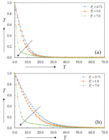
The influence of Prandtl number (Pr = 0.71, 1.0, 7.0) on temperature profile has been depicted in Figures 9a and b at time $\tau$ equal to 20 and 80, respectively. The temperature profile was observed to be smaller for larger value of Prandtl number for both the cases of time 20 and 80. In addition, this temperature profile decreased and reached to zero when the boundary layer thickness (Y) was greater than or equal to 30 (Figure 9a) and 50 (Figure 9b) for the time equal to 20 and 80, respectively. A similar trend of this temperature distribution can be seen in the published works of Pal and Chatterjee [21]; Ali et al. [16] and Thammanna et al. [17].
Figure 9. Temperature profile as a function of Y for different values of Prandtl number (Pr) at times (a) $\tau$ = 20 and (b) $\tau$ = 80. The values of Gr, Gm, $\Delta$, M, Da, Fo, $\Lambda, \lambda$, Df, Ec, Sc and So are equal to 0.2, 1.0, 0.1, 0.2, 1.0, 0.1, 0.5, 0.1, 0.5, 0.1, 0.22 and 0.6, respectively
5.7 Effects of Schmidt number on concentration profile
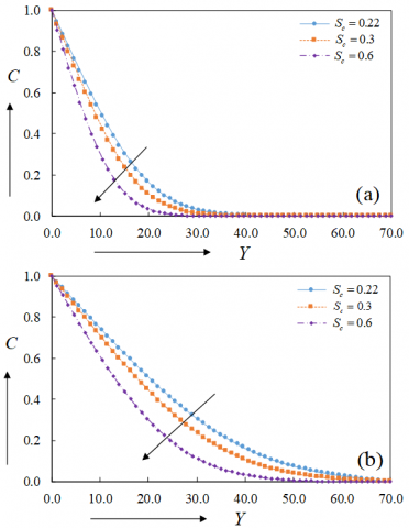
Figures 10a and b show the concentration profile as a function of boundary layer thickness (Y) for different values of Schmidt number (Sc = 0.22, 0.30, 0.66) at time $\tau$ equal to 20 and 80, respectively. A drop in concentration has been noticed when the Schmidt number was increased. In addition, this concentration profile decreased with boundary layer thickness and reached to zero for the case of time $\tau$ = 20 and 80, when Y was greater than or equal to 30 (Figure 10a) and 60 (Figure 10b), respectively.
Figure 10. Concentration profile as a function of Y for different values of Schmidt number (Sc) at times (a) $\tau$ = 20 and (b) $\tau$ = 80. The values of Gr, Gm, $\Delta$, M, Da, Fo, $\Lambda, \lambda$, Pr, Df, Ec, and So are equal to 0.2, 1.0, 0.1, 0.2, 1.0, 0.1, 0.5, 0.1, 0.71, 0.5, 0.1and 0.6, respectively
Transient flow of micropolar fluid on a non-Darcy porous medium in the presence of magnetic field has been investigated numerically in this present work. The explicit finite difference numerical approach has been used as the main tool to solve the dimensionless governing non-linear partial differential equations. The findings have been noted for various values of important parameters such as the Grashof number (Gr), Magnetic parameter (M), Forchheimer number (Fo), Prandtl number (Pr), Spin gradient viscosity parameter (L), Schmidt number (Sc), Vortex viscosity parameter (l). The stability of the system was analyzed, which confirmed that this magnetohydrodynamic system converged for the values of Prandtl and Schmidt number greater than and equal to 0.03. The simulation results demonstrated that the flow pattern changes for the times from 20 to 70. However, the obtained results remained steady when the time reached to the value 75, for all parameters.
The fluid velocity increased for increasing values of Grashof number, however, it decreased for increasing values of magnetic parameter and Forchheimer number. On the other hand, the angular velocity increased when the spin gradient viscosity and vortex viscosity parameter increased. In addition, the Forchheimer number has no effect on the angular velocity. More importantly, the temperature distribution decreased for increasing the values of Prandtl number. Finally, the concentration distribution decreased with Schmidt number. In fact, this research is an important step towards the analysis of micropolar fluid behavior in a non-Darcy porous medium in the presence of magnetic field. The outcome of this study will aid the next level of research work on the analysis of the behavior of micropolar fluid.
The authors would like to thank the Mathematics Discipline, Khulna University, Bangladesh for a support of the fundamental computing lab.
|
u, v, w |
velocity components |
|
x, y, z |
coordinate axis |
|
t |
dimensional time |
|
g |
gravitational acceleration |
|
T |
temperature |
|
C |
concentration |
|
q |
fluid velocity |
|
r |
fluid density |
|
K |
permeability of the porous medium |
|
cb |
constant Forchheimer |
|
j |
microinertia per unit mass |
|
cp |
specific heat at constant pressure |
|
Dm |
coefficient of mass diffusivity |
|
kT |
thermal diffusion ratio |
|
cs |
concentration susceptibility |
|
Tw |
temperature at the plate |
|
$T_{\infty}$ |
uniform fluid temperature |
|
$C_{\infty}$ |
uniform fluid concentration |
|
k |
thermal conductivity of the medium |
|
X |
dimensionless coordinate axis along the plate |
|
Y |
dimensionless coordinate axis normal to the plate |
|
U |
dimensionless velocity along X-axis |
|
V |
dimensionless velocity along Y-axis |
|
U0 |
uniform velocity |
|
$\bar{T}$ |
dimensional temperature |
|
$\bar{C}$ |
dimensional concentration |
|
Gr |
Grashof number |
|
Gm |
modified Grashof number |
|
Pr |
Prandtl number |
|
Sc |
Schmidt number |
|
Da |
Darcy number |
|
F0 |
Forchheimer number |
|
Df |
Dufour number |
|
Ec |
Eckert number |
|
S0 |
Soret number |
|
B0 |
external magnetic field |
|
M |
magnetic parameter |
|
Greek symbols |
|
|
υ |
Kinematic viscosity |
|
μ |
Viscosity of the fluid |
|
χ |
Vortex viscosity |
|
γ |
Spin gradient Viscosity |
|
G |
Angular velocity |
|
σʹ |
Electric conductivity of the fluid |
|
β |
Coefficient of volume expansion |
|
β* |
Coefficient of concentration expansion |
|
$\Delta$ |
Micro-rotation parameter |
|
$\Lambda$ |
Spin gradient viscosity parameter |
|
$\lambda$ |
Vortex viscosity parameter |
|
$\tau$ |
Dimensionless time |
|
$\bar{\Gamma}$ |
Dimensionless angular velocity |
[1] Mahmoud, M.A. (2007). Thermal radiation effects on MHD flow of a micropolar fluid over a stretching surface with variable thermal conductivity. Physica A: Statistical Mechanics and its Applications, 375(2): 401-410. https://doi.org/10.1016/j.physa.2006.09.010
[2] Rahman, M.M., Aziz, A., Al-Lawatia, M.A. (2010). Heat transfer in micropolar fluid along an inclined permeable plate with variable fluid properties. International Journal of Thermal Sciences, 49(6): 993-1002. https://doi.org/10.1016/j.ijthermalsci.2010.01.002
[3] Ahmad, K., Ishak, A., Nazar, R. (2013). Micropolar fluid flow and heat transfer over a nonlinearly stretching plate with viscous dissipation. Mathematical Problems in Engineering, 2013: 1-5. https://doi.org/10.1155/2013/257161
[4] Uddin, M.S., Bhattacharyya, K., Shafie, S. (2016). Micropolar fluid flow and heat transfer over an exponentially permeable shrinking sheet. Propulsion and Power Research, 5(4): 310-317. https://doi.org/10.1016/j.jppr.2016.11.005
[5] Eringen, A.C. (1966). Theory of micropolar fluids. Journal of Mathematics and Mechanics, 16: 1-18.
[6] Gorla, R.S.R. (1988). Combined forced and free convection in micropolar boundary layer flow on a vertical flat plate. International Journal of Engineering Science, 26(4): 385-391. https://doi.org/10.1016/0020-7225(88)90117-6
[7] Gorla, R.S.R. (1992). Mixed convection in a micropolar fluid from a vertical surface with uniform heat flux. International Journal of Engineering Science, 30(3): 349-358. https://doi.org/10.1016/0020-7225(92)90080-Z
[8] El-Hakiem, M.A., Mohammadein, A.A., El-Kabeir, S.M.M., Gorla, R.S.R. (1999). Joule heating effects on magnetohydrodynamic free convection flow of a micropolar fluid. International Communications Heat Mass Transfer, 26(2): 219-227. https://doi.org/10.1016/S0735-1933(99)00008-1
[9] El-Arabawy, H.A. (2003). Effect of suction/injection on the flow of a micropolar fluid past a continuously moving plate in the presence of radiation. International Journal of Heat Mass Transfer, 46(8): 1471-1477. https://doi.org/10.1016/S0017-9310(02)00320-4
[10] Ganesan, P., Palani, G. (2004). Finite difference analysis of unsteady natural convection MHD flow past an inclined plate with variable surface heat and mass flux. International Journal of Heat and Mass Transfer, 47(19): 4449-4457. https://doi.org/10.1016/j.ijheatmasstransfer.2004.04.034
[11] Abo-Eldahab, E.M., Ghonaim, A.F. (2005). Radiation effect on heat transfer of a micropolar fluid through a porous medium. Applied Mathematics and Computation, 169(1): 500-510. https://doi.org/10.1016/j.amc.2004.09.059
[12] Islam, A., Biswas, M.H.A., Islam, M.R., Mohiuddin, S.M. (2011). MHD micropolar fluid flow through vertical porous medium. Academaic Research International, 1(3): 381.
[13] Palani, G., Kim, K.Y. (2011). Joule heating and viscous dissipation effects on MHD flow past a semi-infinite inclined plate with variable surface temperature. Journal of Engineering Thermophysics, 20(4): 501-517. https://doi.org/10.1134/S1810232811040138
[14] Bég, O.A., Rashidi, M.M., Bég, T.A., Asadi, M. (2012). Homotopy analysis of transient magneto-bio-fluid dynamics of micropolar squeeze film in a porous medium: a model for magneto-bio-rheological lubrication. Journal of Mechanics in Medicine and Biology, 12(03): 1250051. https://doi.org/10.1142/S0219519411004642
[15] Haque, M.Z., Alam, M.M., Ferdows, M., Postelnicu, A. (2012). Micropolar fluid behaviors on steady MHD free convection and mass transfer flow with constant heat and mass fluxes, joule heating and viscous dissipation. Journal of King Saud University-EngineeringSciences, 24(2): 71-84. https://doi.org/10.1016/j.jksues.2011.02.003
[16] Ali, L.E., Islam, A., Islam, N. (2015). Investigate micropolar fluid behavior on MHD free convection and mass transfer flow with constant heat and mass fluxes by finite difference method. American Journal of Applied Mathematics, 3(3): 157-168. https://doi.org/10.11648/j.ajam.20150303.23
[17] Thammanna, G.T., Kumar, G.K., Gireesha, B.J., Ramesh, G.K., Prasannakumara, B.C. (2017). Three dimensional MHD flow of couple stress Casson fluid past an unsteady stretching surface with chemical reaction. Results in Physics, 7: 4104-4110. https://doi.org/10.1016/j.rinp.2017.10.016
[18] Bég, O.A., Bég, T.A., Karim, I., Khan, M.S., Alam, M.M., Ferdows, M., Shamshuddin, M.D. (2019). Numerical study of magneto-convective heat and mass transfer from inclined surface with Soret diffusion and heat generation effects: A model for ocean magnetic energy generator fluid dynamics. Chinese Journal of Physics, 60: 167-179. https://doi.org/10.1016/j.cjph.2019.05.002
[19] Haque, M.M. (2021). Heat and Mass Transfer Analysis on Magneto Micropolar Fluid Flow with Heat Absorption in Induced Magnetic Field. Fluids, 6(3). https://doi.org/10.3390/fluids6030126
[20] Zeng, Z., Grigg, R. (2006). A criterion for non-Darcy flow in porous media. Transport in Porous Media, 63(1): 57-69. https://doi.org/10.1007/s11242-005-2720-3
[21] Pal, D., Chatterjee, S. (2012). MHD non-darcy mixed convection stagnation-point flow of a micropolar fluid towards a stretching sheet with radiation. Chemical Engineering Communications,199(9): 1169-1193. https://doi.org/10.1080/00986445.2011.647136
[22] Mohammadien, A.A., El-Amin, M.F. (2000). Thermal dispersion–radiation effects on non-Darcy natural convection in a fluid saturated porous medium. Transport in Porous Media, 40(2), 153-163. https://doi.org/10.1023/A:1006654309980
[23] Murthy, P., Singh, P. (1999). Heat and mass transfer by natural convection in a non-Darcy porous medium. Acta Mechanica, 138(3-4): 243-254. https://doi.org/10.1007/BF01291847
[24] El-Amin, M.F. (2004). Double dispersion effects on natural convection heat and mass transfer in non-Darcy porous medium. Applied Mathematics Computation, 156(1): 1-17. https://doi.org/10.1016/j.amc.2003.07.001
[25] Noghrehabadi, A., Behseresht, A., Behseresht, M.G. (2013). Natural-convection flow of nanofluids over vertical cone embedded in non-Darcy porous media. Journal of Thermophysics Heat Transfer, 27(2): 334-341. https://doi.org/10.2514/1.T3965
[26] El-Dabe, N., Shaaban, A.A., Abou-Zeid, M.Y., Ali, H.A. (2015). Magnetohydrodynamic non-Newtonian nanofluid flow over a stretching sheet through a non-Darcy porous medium with radiation and chemical reaction. Journal of Computational Theoretical Nanoscience, 12(12): 5363-5371. https://doi.org/10.1166/jctn.2015.4528
[27] Seth, G.S., Kumar, R., Tripathi, R. Bhattacharyya, A. (2018). Double diffusive MHD Casson fluid flow in a non-Darcy porous medium with Newtonian heating and thermo-diffusion effects. International Journal of Heat Technology, 36(4): 1517-1527. https://doi.org/10.18280/ijht.360446
[28] Callahan, G.D., Marner, W.J. (1976). Transient free convection with mass transfer on an isothermal vertical flat plate. International Journal of Heat and Mass Transfer, 19(2): 165-174. https://doi.org/10.1016/0017-9310(76)90109-5
[29] Soundalgekar, V.M., Ganesan, P. (1981). Finite-difference analysis of transient free convection with mass transfer on an isothermal vertical flat plate. International Journal of Engineering Science, 19(6): 757-770. https://doi.org/10.1016/0020-7225(81)90109-9