Kamaran K.F. Rashid | Idres I.A. Hamakhan* | Chalang C.H. Mohammed
© 2022 IIETA. This article is published by IIETA and is licensed under the CC BY 4.0 license (http://creativecommons.org/licenses/by/4.0/).
OPEN ACCESS
The goal of this study is to investigate the heat transfer as well as optimizing the tilt angle of an active flat plate solar collector. In addition, MATLAB software is used for study the flat plate solar performance of the collector. The entire test rig, with a complete control system, has been set up to collect practical data in September and October 2021. The results showed that the collector efficiency rises with the usable heat rate, peaking at 77% in the autumn (14 October) at the optimal heat rate of 975 W and an outlet water temperature of 64℃. However, the system efficiency for the sunny environment is 53% with an outlet temperature of 36℃ in winter (6 Jan). According to this investigation, the monthly average value and yearly value of optimum tilt angle were found to be 30° to 40° and 30°, respectively, for Erbil climate conditions. Also, this study reveals that the average heat loss coefficient between theoretical models and experimental work was 4.352 W/m2.℃. Furthermore, the temperature difference, corresponding to the same amount of heat loss coefficient, was 14.4℃ for the practical model but 15.25℃ for the theoretical part. This study proposes that using the entire experimental data from a Flat Plate Solar Collector instead of using average values and comparing it to the mathematical equations implemented in the MATLAB software, the thermal efficiency of the system was increased by 5%.
heat transfer, tilt angle, performance analysis, active flat plate solar collector
In many nations now, developments in the quality of life, in addition to fast progress, are driving higher energy consumption, and the possibility of a future imbalance between demand and supply is expected to be enormous [1]. As a result, the topic of long-term growth is gaining traction. Renewable energy is gaining popularity due to its inherent sustainability and environmental friendliness. Renewable energy has been incorporated as a key source of energy in the energy plans of all industrialized nations and many developing countries [2]. The new climate change law [3] established a goal of a 60% reduction by 2050. Little and nil carbon technologies offer the ability to address major concerns about sustainable development's economic, ecological, and social difficulties [4].
Solar energy has received particular attention among the numerous types of renewable energy since it is readily accessible. As the world's energy supplies have depleted, the motivation to create solar energy solutions has grown. As a result, research into solar energy uses has exploded, taking advantage of solar energy's plentiful, free, and ecologically friendly properties. At present, the primary aspect of this study is to save approximately 1383 KWh of energy per year. The second goal is to reduce annual CO2 emissions by approximately 781 kg per one FPSC.
Energy coming from the sun is crucial in modernized countries because electricity is costly, plus energy output is insufficient to fulfill demand. Solar energy is the excellent alternate energy basis because it is plentiful, unlimited, and non-poisoning. Dissimilar oil reserves, in addition to mineral resources, which are prone to reduction in the near future [5, 6], are for free-tip of the environment that is not subject to upcoming reduction.
Solar thermal structures, for example, solar water warmers, air warmers, ovens, dryers, and condensation equipment, have made significant progress in terms of efficiency and dependability during the last several decades. The use of insulation materials, the control system and organization using sensors, actuators, and control units, and the optimization of the tilt angle are the most important parameters to improve efficiency and reliability. At low- and moderate-temperature approaches, these devices' efficiencies generally range from 40 to 60 percent [7]. The solar accumulator is the most crucial part of the scheme because it converts solar energy into warmth and then transmits that warmth to a working liquid for use in a finish-usage system. Solar collectors are generally classified into two types: concentrating as well as the flat plate solar collectors. Depending on a temperature variety needed, the focused collector can track solar radiation with or without tracking solar. They only work with direct sunlight and are only functional on days when the sky is clear. The flat plate solar collectors (FPSC) have the benefit of catching both diffused and beam solar radiation, so it may continue to work even when the sun is blocked by a cloud [8, 9].
The flat-plate collector's optimal orientation is normally set, and it's ideal for applications that need energy delivery at temperatures below 100℃ higher than ambient [10, 11]. A (FPSC) linked above the heat pipelines, through which freshening water runs and takes out heat from the collector, is the most common form of household solar hot water arrangement with heat tubing. Water travels between the flat-plate collector as well as the thermal tank, which stores the heat received from the collector [12]. The FPC is fixed within a container with a clear glass cover at the top. This layout is designed to reduce heat losses. Because of their dependable performance, low price, low repairs, and ease of arrangement with building facades, Thermosyphon household solar liquid warmers (FPSC) have been frequently used in housing and business construction for water, in addition to space warming [13].
Many investigations [14] use a rectangular narrow ducting absorber type (FPSC). They came to the conclusion that rectangular ducting absorbers may significantly enhance the collector's thermal performance, but at a higher cost due to the increased consumption of electric pumping energy.
A comparison study of theoretic guesses and practical findings of (FPSC) with heating pipelines was conducted by Ismail and Abogderah [15]. The heating pipeline solar collector's theoretical model was created using Beckman and Duffie’s technique [16], but it was changed to employ heat pipes for energy delivery. According to their findings, the heating pipeline solar collector's immediate efficiencies are lower than traditional collectors in the morning and are also greater when heating pipelines reach their operational temperature.
Facao and Oliveira [17] investigated the thermal behavior of the FPSC heating pipeline experimentally. A temperature in the heating pipeline was assumed to be constant and identical to fullness temperatures, which was a significant simplification. Their findings for a non-selective surface coating indicated the collector's visual efficiency (64%) as well as the overall loss coefficient (5.5 W/m2K).
Several research studies, as described above, have examined the impact of different collector absorber schemes on heating transmission and solar water heating system performance. According to current research, the flat plat solar collector is the best for home applications, but it requires tilt angle organization, an efficient control unit, and the construction of the FPSC’s glass layer.
Heat transmission in the solar collector using liquid waterway tubes across its size was studied both in theory and empirically in this work. A collector and connected pipelines controlling equations were provided. A mathematical model in this study drives away from equation energy balance to include equation heat transfer for components of the collector. The efficiency of collectors, exit liquid temperature, and heat loss from the structure were all calculated using theoretical calculations. It's an attractive technical option for producing hot water in rural locations because of its ease of manufacture and lack of moving components.
The first target of this paper is to investigate the performance analysis of an active flat plate solar collector based on experimental data and compare it to various theoretical equations. The test rig was built in a real-world atmosphere to collect useful data about Erbil's climate conditions. The second aim is to optimize the tilt angle for the entire year. The MATLAB software was used for this.
2.1 Mathematical formulation
It is appropriate to develop a computer model technique to studies the impact of parameters on a performances of a flat plate solar collector. This process is established by finding a solar energy attainment on tilt surface of a collector in addition to actually determining the valuable energy achievement by calculating losses [18]. The technique is defined as follows: This equation [18] May be used to compute the total solar energy radiation achievement of a horizontally tilted surface slope north-south as well as facing the equator.
$I_{T}=I_{D N}\left[\cos \theta+C\left(\frac{1+\cos \beta}{2}\right)+\rho_{g}(C+\sin \theta)\left(\frac{1+\cos \theta}{2}\right)\right]$ (1)
This includes both direct as well as diffuse radiation, as well as radiation from earth.
$I_{D N}=A \exp \left(\frac{-B}{\sin \emptyset}\right)$ (2)
A, B, as well as C are fixed, although their values fluctuate over the year. In the study of ref. [19] specifies these standard values for every month of a year.
The sun's angle of altitude $\varnothing$ and incident angle θ can be calculated using the calculations stated in the study of ref. [20] as
$\sin \emptyset=\cos \delta \cos L \cos h+\sin \delta \sin L$ (3)
$\cos \theta=\cos (L-\beta) \cos \delta \cos h+\sin (L-\beta) \sin \delta$ (4)
$\delta=23.45 \sin \left[\frac{360}{365}(284+D N)\right]$
$h=(15.0) T$ (5)
While DN is just a number of the day in a year beginning on January 1st.
The technique provided by Duffie and Beckman [18] may be used to compute all of a solar energy absorbed by a collector as
$\begin{aligned} S=I_{D N}\left[(\tau \alpha)_{D} \cos \theta\right.&+(\tau \alpha)_{D S} C\left(\frac{1+\cos \beta}{2}\right) \\+&\left.(\tau \alpha)_{D G} \rho_{g}(C+\sin \emptyset)\left(\frac{1-\cos \beta}{2}\right)\right] \end{aligned}$ (6)
where, $(\tau \alpha)_{D}$ is direct solar radiations given by applying the next arrangement of the formulae [15].
$(\tau \alpha)_{D}=\left[\left(\frac{\tau \alpha}{1-\alpha}\right) \rho_{d}\right]$ (7)
$\tau=\tau_{r} \tau_{a}$ (8)
$\tau_{r}=\frac{1}{2}\left(\left\{\frac{\left(1-r_{1}\right)}{\left[1+(2 N G-1) r_{1}\right]}\quad\right\}+\left\{\frac{\left(1-r_{2}\right)}{\left[1+(2 N G-1) r_{2}\right]}\quad\right\}\right)$ (9)
$\tau_{a}=\exp \left(-K N G \frac{\delta_{g}}{\cos \theta_{1}}\right)$ (10)
$r_{1}=\left[\frac{\sin \left(\theta_{1}-\theta\right)}{\sin \left(\theta_{1}+\theta\right)}\right]^{2}$ (11)
$r_{2}=\left[\frac{\tan \left(\theta_{1}-\theta\right)}{\tan \left(\theta_{1}+\theta\right)}\right]^{2}$ (12)
$\theta_{1}=\sin ^{-1}\left(\frac{\sin \theta}{n}\right)$ (13)
$\rho_{d}=\tau_{a}-\tau$ (14)
The α absorber plate's absorptivity is believed to remain constant. The product transmittance-absorptance of the sky plus ground diffuse radiation are calculated in the same way, with the exception that in direct radiation, the incidence angle $\theta$ is substituted by the effective incidence angles $\theta_{e}$ in the corresponding situations, by Duffle plus Beckman's relations. [18] As,
$\theta_{e S}=59.68-0.1388 \beta+0.001497 \beta^{2}$ (15)
$\theta_{e g}=90-0.5778 \beta+0.002693 \beta^{2}$ (16)
After accounting for different losses from the collector, the usable energy gathered by the collector is calculated using the following approach [18]. In Figure 1 shown important parameters of FPSC system.
$Q_{u}=F_{R}\left[S-U_{L}\left(T_{f i}-T_{a}\right) A_{c}\right]$ (17)
where, $S=\tau \alpha \mathrm{I}_{\mathrm{t}} \mathrm{A}_{\mathrm{c}}$, so $F_{R} A_{c}\left[\alpha \tau I_{T}-U_{l}\left(T_{f i}-T_{a}\right)\right]$.
$F_{R}=F^{\prime} * F^{\prime \prime}$ (18)
$F^{\prime}=\frac{(W-D) F+D}{W\left[1+\frac{U_{L}(W-D) F+D}{\pi D_{i} h_{i}}\right]}$ (19)
$F^{\prime \prime}=\frac{\dot{m}_{w} C_{p}}{A_{c} U_{L} F^{\prime}}\left\{1-\exp \left[-\left(\frac{A_{c} U_{L} F^{\prime}}{\dot{m}_{w} C_{p}}\right)\right]\right\}$ (20)
$F=\frac{\tanh [\mathrm{m}(\mathrm{w}-\mathrm{D}) / 2]}{\mathrm{m}(\mathrm{w}-\mathrm{D}) / 2}$ (21)
$\mathrm{m}=\sqrt{\frac{\mathrm{U}_{\mathrm{L}}}{K_{p} \delta_{p}}}$ (22)
$h_{i}=\frac{N_{u} K_{w}}{D_{i}}$ (23)
$\left\{\begin{array}{c}N_{u}=4.36 \text { for laminar flow } \\ N_{u}=0.023 R e^{0.8} P^{0.33} \text { for turbulent flow }\end{array}\right\}$ (24)
The characteristics of water driven at the particular fluid mean temperature:
$T_{f m}=T_{f i}+\frac{Q_{u}}{\left(2 m_{w} c_{p}\right)}$ (25)
Many researchers have developed correlations for estimating a coefficient of heat loss UL, including [18, 21], and [22], and their exertion is discussed in Reference [22]. The coefficient of heat loss UL is determined in this study utilizing the relationship described in the reference [18], as
$\mathrm{U}_{\mathrm{L}}=\mathrm{U}_{\mathrm{T}}+\mathrm{U}_{\mathrm{B}}$ (26)
$\mathrm{U}_{\mathrm{T}}$$=\left[\frac{\mathrm{NG}}{\frac{\mathrm{C}}{\mathrm{T}_{\mathrm{pm}}}\left[\frac{\left(\mathrm{T}_{\mathrm{pm}}-\mathrm{T}_{\mathrm{a}}\right)}{(\mathrm{NG}+\mathrm{f})}\right]^{\mathrm{e}}}+\frac{1}{\mathrm{~h}_{\mathrm{w}}}\right]^{-1}$ $+\frac{\sigma\left(\mathrm{T}_{\mathrm{pm}}+\mathrm{T}_{\mathrm{a}}\right)\left(\mathrm{T}_{\mathrm{pm}}^{2}-\mathrm{T}_{\mathrm{a}}^{2}\right)}{\left(\varepsilon_{\mathrm{p}}+0.00591 \mathrm{Nh}_{\mathrm{w}}\right)^{-1}+\frac{2 \mathrm{NG}+\mathrm{f}-1+0.133 \varepsilon_{\mathrm{p}}}{\varepsilon_{\mathrm{g}}}-\mathrm{NG}}$ (27)
$\mathrm{f}=\left(1+0.089 \mathrm{~h}_{\mathrm{w}}-0.1166 \mathrm{~h}_{\mathrm{w}} \varepsilon_{\mathrm{p}}\right)(1+0.07866 \mathrm{~N})$
$\mathrm{C}=250\left(1-0.000051 \beta^{2}\right)$ for $0^{\circ}<\beta<70^{\circ}$
$\mathrm{e}=0.43\left(1-\frac{100}{\mathrm{~T}_{\mathrm{p}, \mathrm{m}}}\right)$
$h_{w}=5.7+3.8 U_{m}$
$T_{p m}=T_{f i}+\frac{Q_{u}\left(1-F_{R}\right)}{U_{L} A_{C} F_{R}}$ (28)
$\mathrm{U}_{\mathrm{B}}=\frac{1}{\mathrm{R}}=\frac{K_{i}}{\delta_{i}}$ (29)
The determination of Qu requires an understanding of UL, which is dependent on the plate mean temperature. According to Eq. (17), as shown above, there is an inverse relationship between them, with decreasing the value of UL causing an increase in the value of Qu. Only the values of Qu and UL may be used to calculate the plate mean temperature. As a result, using the iterative technique to find Qu is critical. First, a reasonable mean plate temperature was supposed, as well as at that time UL plus Qu are calculated using formulas (26) plus (27) respectively. Once Qu is determined, Eq. (28) is used to compute the plate mean temperature, which is then compared to the supposed value. If a major difference between both the calculated as well as supposed value of mean temperature of plate is not with the acceptable precision, the computation is redone using a new assuming value of Tpm as that of the typical of a previously computed and supposed value of mean plate temperature. This method is repeated till the assumed and computed values are within the acceptable accuracy range.
Figure 1. FPSC with liquid pipelines is shown schematically
2.2 Simulation process
Table 2 shows the parameters that have been set to control the dynamic simulation in a basic simulation the following thermal models can be used for Flat plate Solar collector: Eqns. (30), (31), (32), and (33) can be used to calculate the collection fluid output temperature and efficiency:
$\mathrm{T}_{\mathrm{fo}}=\mathrm{T}_{\mathrm{fi}}+\frac{\mathrm{Q}_{\mathrm{u}}}{\dot{\mathrm{m}} \mathrm{C}_{\mathrm{pf}}}$ (30)
$\mathrm{Q}_{\mathrm{u}}=\mathrm{A}_{\mathrm{c}} \mathrm{F}_{\mathrm{R}}\left[\tau \alpha \mathrm{I}_{\mathrm{t}}-\mathrm{U}_{\mathrm{L}}\left(\mathrm{T}_{\mathrm{fi}}-\mathrm{T}_{\mathrm{a}}\right)\right]$ (31)
$\mathrm{F}_{\mathrm{R}}=\frac{\dot{\mathrm{m}} \mathrm{C}_{\mathrm{pf}}}{\mathrm{A}_{\mathrm{c}} \mathrm{U}_{\mathrm{L}}}\left(1-\mathrm{e}^{\frac{-\mathrm{A}_{\mathrm{c}} \mathrm{U}_{\mathrm{L}} \mathrm{F}^{\prime}}{\mathrm{\textrm {m }} \mathrm{pf}_{\mathrm{pf}}}}\right)$ (32)
$\eta_{c}=\frac{Q_{u}}{A_{c} I_{t}}$ (33)
2.3 Optimizing the tilt angle
To be able to receive the most solar radiation rays through the drying seasons, solar collectors are oriented nearly perpendicular to the energy rays. Within a year, the tilt angle will change with the change in the sun's illumination angle, but the optimum value of the tilt angle over the year or per dry season must be determined.
The collector achieves the best thermal performance all year when it is facing south in the northern hemisphere [23]. The collectors' slope allows for easy water drainage and improves air circulation [6]. This study used the tilt angle optimization equation, which is based on a model developed by Reindl et al. [24] and Kim et al. [25]. Table 2 shows the parameters that have been set to control the dynamic simulation and optimization.
$\begin{aligned} \mathrm{H}_{\mathrm{T}}=\left(\mathrm{H}_{\mathrm{b}}+\mathrm{H}_{\mathrm{d}} \mathrm{A}_{\mathrm{i}}\right) \mathrm{R}_{\mathrm{b}} &+\mathrm{H}_{\mathrm{b}}\left(1-\mathrm{A}_{\mathrm{i}}\right)\left(\frac{1+\cos \beta}{2}\right)\left[1+\mathrm{fsin}^{3} \frac{\beta}{2}\right] \\ &+\mathrm{H}\left(\frac{1-\cos \beta}{2}\right) \end{aligned}$ (34)
$\left(\mathrm{H}_{\mathrm{b}}\right)$ On horizontal surface total beam radiation.
$(\beta)$ Angle of tilt collector.
(H) On horizontal surface monthly daily’s solar radiations.
$\left(\mathrm{H}_{\mathrm{d}}\right)$ Total diffuse radiation on the horizontal surface.
$\left(\mathrm{H}_{\mathrm{T}}\right)$ On the tilted surface solar radiation.
$\left(A_{i}\right)$ Is the anisotropic index.
$A_{\mathrm{i}}=\frac{\overline{\mathrm{H}}_{\mathrm{b}}}{\overline{\mathrm{H}}_{\mathrm{o}}}$ (35)
$\mathrm{f}$ is square root ratio of the beam to the total radiation specified as:
$\mathrm{f}=\left(\frac{\mathrm{H}_{\mathrm{b}}}{\mathrm{H}}\right)^{1 / 2}$ (36)
The beam component may be founding by:
$\mathrm{H}_{\mathrm{b}}=\mathrm{H}-\mathrm{H}_{\mathrm{d}}$ (37)
$\mathrm{R}_{\mathrm{b}}$ is a geometric factor.
$\mathrm{R}_{\mathrm{b}}=\frac{\cos (\varphi-\beta) \cos \delta \sin \omega_{\mathrm{s}}^{\prime}+\left(\frac{\pi}{180}\right) \omega_{\mathrm{s}}^{\prime} \sin (\varphi+\beta) \sin \delta}{\cos \varphi \cos \delta \sin \omega_{\mathrm{s}}^{\prime}+\left(\frac{\pi}{180}\right) \omega_{\mathrm{s}}^{\prime} \sin \varphi \sin \delta}$
$\omega_{\mathrm{s}}^{\prime}=\min$
$\cos ^{-1}(-\tan \varphi \tan \beta)$
$\cos ^{-1}(-\tan (\varphi+\beta) \tan \delta)$ (38)
Means the lesser of two values in brackets, $\left(\omega_{s}\right)$. The angle of the sunset hour is determined by:
$\omega_{s}=\cos ^{-1}\left(-\tan ^{-1} \varphi \tan ^{-1} \delta\right)$ (39)
( $\varphi)$ Latitude of a location
( $\delta$ ) Angle of declination
$\delta=23.45 \sin \left[\frac{360}{365}(284+\mathrm{DN})\right]$ (40)
(DN) Number of days in the year and can be obtained using Table 1.
2.4 Experimental setup
Figure 2 depicts the flat-plate solar collector practical configuration. The temperatures of the collector's input and outflow river, and an ambient temperature and liquid inside the tank, were measured using a K-type thermocouple with standard error limits of 2.2℃ and a water flow sensor range of 1-30 L/min (flow meter model YF-S201), G1/2 Black. In the standard case, the liquid flow rate is within the margin of error (3 percent). After factory calibration, the solar radiation was measured with a LI-19 read-out unit and a data logger with µV sensitivity and a basic accuracy of 0.1 percent.
This system was tested for 30 days in September and October 2021, with readings taken every 7 hours between 9 a.m. and 4 p.m. Water was being supplied by a collector from the lowest level of a storage reservoir. The water's achieved inlet temperature ranges between 25 and 60℃. The obtained data was used to calculate system performance parameters using the above-mentioned equations.
Table 1. Values of DN by Months [18]
|
Months |
DN for ith Day of the months |
Dates |
DN, Day of the Year |
The Declination |
|
January |
i |
17 |
17 |
-20.9 |
|
February |
31+i |
16 |
47 |
-13 |
|
March |
59+i |
16 |
75 |
-2.4 |
|
April |
90+i |
15 |
105 |
9.4 |
|
May |
120+i |
15 |
135 |
18.8 |
|
June |
151+i |
11 |
162 |
23.1 |
|
July |
181+i |
17 |
198 |
21.2 |
|
August |
212+i |
16 |
228 |
13.5 |
|
September |
243+i |
15 |
258 |
2.2 |
|
October |
273+i |
15 |
288 |
-9.6 |
|
November |
304+i |
14 |
318 |
-18.9 |
|
December |
334+i |
10 |
344 |
-23 |
Table 2. List of parameters to control the dynamic simulation and optimizations
|
Parameter |
Value |
|
Gross area m2 |
1,81 |
|
Tilt angle |
40° |
|
Mass flow rate(L/M) |
2 |
|
Bottom thickness mm |
0,40 |
|
Absorbance |
95% |
|
Emittance |
3% |
|
Diameter of absorber tube (D) mm |
12 |
|
Absorber thickness mm |
0,20 |
|
Number of tube |
10 |
|
Tube pitch (W) mm |
86 |
|
Transmittance of glass |
91 % |
|
Thickness of glass mm |
4 |
|
Thermal conductivity W/m2.K |
0.037 |
|
Thickness of wool mm |
50 |
|
Absorber tube wall thickness mm |
0,50 |
|
Absorber and pipe material |
Copper |
|
day of the year DN average |
228 |
|
monthly average daily solar radiation, on a horizontal surface (H) Kwh/m2 |
7.37 |
|
diffuse total radiation on a horizontal surface (Hd)kwh/m2 |
1.474 |
|
total beam radiation, on a horizontal surface (Hb) kwh/m2 |
5.896 |
|
Declination angle, $\delta$ |
13.56 |
|
Latitude, $\varphi$ |
36.2191 |
Figure 2. Experimental setup for the water heating solar system
3.1 Numerically and experimentally measured data
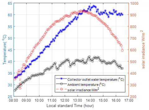
Figure 3 depicts a typical daytime change in ambient temperature, output water temperature, and solar radiation. The findings reveal that the maximum liquid temperature reached is the function of both ambient air temperature and solar radiation. As shown in Figure 3, and from the MATLAB simulation curve that an increase in both variables is a specific cause of the increase in water temperature. When the sun was shining brightly, the collector's energy output was highest around midday, and it was lowest in the mornings and afternoons.
Throughout the test, the highest outgoing liquid temperature of 64℃ was found. With a highest temperature in the environment of 41℃ for the day, at around 14.00 h of the day, the hot liquid temperature is 23℃ higher than the ambient temperature. A large temperature differential is achieved as a consequence of a system's effective insulation.
Figure 4 depicts the curves of the collector's theoretical as well as experimental coefficients of heat loss as the function of a temperature differential between ambient temperature (Ta) and output water temperature (Tco). A heat loss coefficient changes mostly with the temperature gradient; the heat loss coefficient rises when the temperature difference rises, because the ambient air temperature is frequently lower than the temperature of the water, which is a reason for transferring heat from the solar collectors to the surrounding air. As a result, we must maintain the temperature of the water close to the surrounding air by drawing heat from the water coming out of the solar panel, which can also be approved by Eq. (17). The rate of heat loss from the system increases as the temperature differential between the temperature of the collector and the temperature of the surrounding environment increased. When the temperature differential is between 5 and 28℃, the collector's heat loss coefficient changes from 3.12 to 4.67 W/m2℃. Although the experimental values were slightly out of whack, the theoretical and experimental findings were in good agreement. The disparities could be attributed to the computational assumptions used as well as the measurement precision.
The average coefficient of heat loss of 4.352 (W/m2℃) was discovered during the experiment, and the temperature difference at this value (Tco – Ta) was 14.5℃, whereas it was 15.25℃ in the theoretical analysis.
Figure 3. The hourly variations in outlet water and ambient temperature and solar radiation over a typical day
Figure 4. Heat loss coefficients as a function of the difference temperatures among outputs water as well as ambient temperatures (Tco – Ta)
Figure 5 depicts the theoretical plus experimental findings of the solar collector's useable heat rate as a function of time. But after 14 o'clock, the heat rate dropped sharply, that occurred because the use of water output was temporarily halted in order to assess how water circulation affected system performance. As a result, the heat rate dropped dramatically. The useable heat rate has reached its peak. around midday, when a collector gets the most energy, while it is at its lowest both early in the morning and late in the afternoon, owing to little solar radiation through these times. When comparing Figures 3 and 5, it's clear that the usable heat rate is the function of solar radiation; as solar radiation rises, the valuable heat rate produced by a collector rises as well. Furthermore, the discrepancy between theoretical and actual findings in the mornings and afternoons is owing to the sun's angle of incidence at these times, which hinders the collector's functioning. Aside from that, A theoretical as well as experimental findings were in good arrangement.
Figure 5. Variation in the solar collector's useable heat rate with time
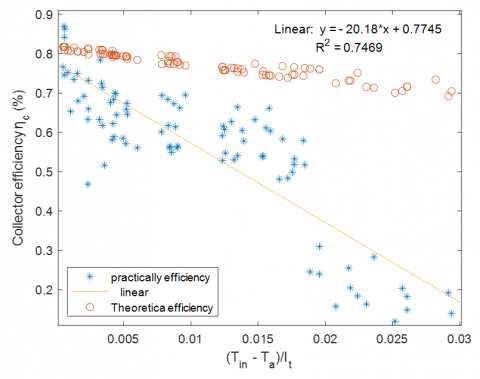
Figure 6 shows how the collector efficiency varies with a collector’s performances coefficient (Tci – Ta) /I. As the collector efficiency decreases, a collector performance coefficient increases, as seen in this diagram. An increase in the temperature differential (Tci – Ta) will increase the collector performance coefficient as well as the collector's heat losses, lowering collector efficiency. The curves also show a high level of agreement among theoretical as well as practical results.
Figure 7 illustrates the experimental efficiency of the solar collector as a function of heat rate. As the heat rate rises, the collector's performance improves until it reaches its maximum value.
Figure 6. Collector efficiency as a function of collector performance coefficient (Tci – Ta)/I
Later which any future rise in a heat rate takes almost no effect on the collector's performance. At an optimal heat rate of (975) W, a maximum efficiency of 77% was achieved during the test.
Figure 7. The solar collector's efficiency varies with the heat rate in local standard time
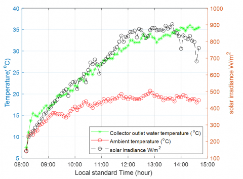
Figure 8. In the winter, hourly changes in ambient temperature, collector-outlet water temperature, and sun radiation (6 Jan)
The data obtained for the winter of January 6th is depicted in Figure 8. According to the graph, the maximum outlet water temperature is 36 degrees Celsius, with the highest ambient temperature of 21 degrees Celsius, and the system efficiency is 53% in sunny weather environments.
3.2 Optimum tilt angle
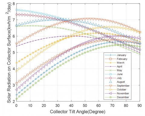
The equations for finding the optimum tilt angles were tested in MATLAB software to investigate the dynamic simulation of the active FPSC for Erbil climate conditions. The block diagram of this simulation is shown in Figure 11. To optimize the tilt angle and output solar rations of the yearly fixed mount FPSC, the tilt angle was changed from 0 to 90 degrees in 1 degree increments, and the solar ration output energy was measured at each angle using the FPSC modeling tool. The result showed that the obtained average monthly optimal tilt angle varies between 30° and 40°. The data also shows that the lowest ideal tilt angle occurred in June and July, while the maximum optimum tilt angle occurred in December, as illustrated in Figure 9 and Table 3. From Figure 10 and Table 4, the yearly optimum tilt angle was 30℃ and the solar insolation collected on the flat plate collector is 7.022 kWh/m2/day.
Figure 9. Optimization of the tilt angle for each month with average days of the months in Table 1
Table 3. Regular optimum monthly tilt angle with irradiation solar energy production for each month
|
Month |
Optimum tilt angle for each month |
Solar Max. value at optimum angle for each month (kwh/m2/day) |
|
January |
76° |
5.651 |
|
February |
70° |
5.775 |
|
March |
60° |
6.182 |
|
April |
40° |
6.009 |
|
May |
10° |
6.634 |
|
June |
0° |
7.61 |
|
July |
0° |
7.32 |
|
August |
30° |
7.023 |
|
September |
54° |
7.063 |
|
October |
68° |
6.564 |
|
November |
74° |
6.011 |
|
December |
78° |
5.459 |
Table 4. The outcome of tilt angle optimization
|
Tilt angle |
Solar radiation Kwh/m2 /day |
|
0° |
5.583 |
|
30° |
7.022 |
|
60° |
6.63 |
Figure 10. Yearly optimization of the tilt angle with recommended average day of the year
Figure 11. The General block diagram optimization and simulation of the tilt angle in MATLAB program expresses the equations no. 34 to 40
This work investigated the theoretical and practical heat transfer and tilt angle optimization for the active flat plat solar collector. The following conclusions have been reached:
|
FPSC |
flat plat solar collector |
|
A |
solar apparent radiation (kJ/h m2) |
|
Ac |
area of collector (m2) |
|
B |
coefficient of atmospheric extinction |
|
C |
The ratio of diffuse to the direct normal radiation |
|
Cp |
water heat capacity c (kJ/kg°C) |
|
Do- Di |
Outer, inner diameters of tubes in side solar collector (m) |
|
DN |
Day of years |
|
F, F', F" |
Collector's fin-efficiency, efficiency-factor, and flow-factor |
|
FR |
Removal heat factors |
|
FR |
Removal heat factors (kg/m2s) |
|
h |
Hours angles |
|
hi, hw |
inside tube and wind convective heat transfer coefficient |
|
IT |
on collector tilt surface total falling solar radiation (kJ/h m2) |
|
IDN |
solar radiation direct normal (kJ/hm2) |
|
K |
glass Absorption coefficient (m-1) |
|
Ki, Kp, Kw |
Thermal conductivity’s; insulation, plate, working fluid (kJ/hm℃) |
|
L |
Latitude angle |
|
ṁw |
flow rate of Mass (kg/s) |
|
n |
glass Refractions index |
|
NG |
glass cover Numbers |
|
Nu |
Nusselt numbers (hi Di/Kw) |
|
Pr |
Prandtl numbers (μw Cp/Kw) |
|
Re |
Reynold numbers (GW Di/μw) |
|
Qu |
energy useful collected (GW Di/μw) |
|
r1, r2 |
in two polarization axes Reflectivity’s |
|
S |
absorbed Solar radiation by absorber of collector (kJ/h) |
|
T |
Time (h) |
|
Ta, Tfi, Tpm |
atmospherics, inlet fluid, mean plate; Temperature (K) |
|
Tfm |
mean temperature of fluid (°C) |
|
UB, UL, UT |
bottom, overall, top; Collectors loss coefficient (kJ/hm2°C) |
|
W |
distance among tubes center point -to-center (m) |
|
Greek symbols |
|
|
$a$ |
absorptance of plate |
|
$\boldsymbol{\beta}$ |
tilt angle of collector (degree) |
|
$\boldsymbol{\delta}$ |
declination angle (degree) |
|
$\boldsymbol{\delta}_{g}, \boldsymbol{\delta}_{i}, \boldsymbol{\delta}_{p}$ |
glass covers, insulations, plate; Thickness (m) |
|
$\epsilon_{g}, \epsilon_{p}$ |
glass, plate; Emissivity’s (degrees) |
|
$\emptyset$ |
altitude angle of the sun |
|
$\mu_{W}$ |
water Dynamic viscosity (kg/ms) |
|
$\rho_{g}$ |
reflectivity Ground surface |
|
$\boldsymbol{\tau}$ |
r transmittance of Cove |
|
$\boldsymbol{\tau}_{\boldsymbol{r}}, \boldsymbol{\tau}_{\boldsymbol{a}}$ |
owing to; reflection, absorption; Cover transmittance |
|
$(\tau \alpha)_{D},(\tau \alpha)_{D G}$ ,$(\tau \alpha)_{D S}$ |
direct, ground diffused, sky diffused; Transmittance- absorptance products |
|
$\boldsymbol{\theta}$ |
Incident angle (degree) |
|
$\theta_{1}$ |
sun beam radiations angle Refracted (degree) |
|
$\boldsymbol{\theta}_{e g}, \boldsymbol{\theta}_{e s}$ |
ground diffused radiations, sky diffused radiations; effective incidence angle |
[1] Kumar, R., Rosen, M.A. (2011). A critical review of photovoltaic–thermal solar collectors for air heating. Applied Energy, 88(11): 3603-3614. http://dx.doi.org/10.1016/j.apenergy.2011.04.044
[2] Eltawil, M.A., Samuuel, D. (2007). Vapour compression cooling system powered by solar PV array for potato storage. https://www.researchgate.net/publication/228348665_Vapour_Compression_Cooling_System_Powered_By_Solar_PV_Array_for_Potato_Storage.
[3] Meadowcroft, J. (2009). Climate change governance. World Bank Policy Research Working Paper, no. 4941. http://dx.doi.org/10.1596/1813-9450-4941
[4] Garnier, C., Currie, J., Muneer, T. (2009). Integrated collector storage solar water heater: Temperature stratification. Applied Energy, 86(9): 1465-1469. http://dx.doi.org/10.1016/j.apenergy.2008.12.009
[5] Alvarez, A., Cabeza, O., Muñiz, M., Varela, L. (2010). Experimental and numerical investigation of a flat-plate solar collector. Energy, 35(9): 3707-3716. http://dx.doi.org/10.1016/j.energy.2010.05.016
[6] Bolaji, B.O., Olalusi, A.P. (2008). Performance evaluation of a mixed-mode solar dryer. https://www.researchgate.net/publication/262213879_Performance_Evaluation_of_a_Mixed-Mode_Solar_Dryer.
[7] Thirugnanasambandam, M., Iniyan, S., Goic, R. (2010). A review of solar thermal technologies. Renewable and Sustainable Energy Reviews, 14(1): 312-322. http://dx.doi.org/10.1016/j.rser.2009.07.014
[8] Vaidya, V., Walke, P., Kriplani, V. (2011). Effects of wind shield on performance of solar flat plate collector. Int. J. Appl. Eng. Res, 6: 379-389.
[9] Momin, A.M.E., Saini, J., Solanki, S. (2002). Heat transfer and friction in solar air heater duct with V-shaped rib roughness on absorber plate. International Journal of Heat and Mass Transfer, 45(16): 3383-3396. https://doi.org/10.1016/S0017-9310(02)00046-7
[10] Huang, J., Pu, S., Gao, W., Que, Y. (2010). Experimental investigation on thermal performance of thermosyphon flat-plate solar water heater with a mantle heat exchanger. Energy, 35(9): 3563-3568. http://dx.doi.org/10.1016/j.energy.2010.04.028
[11] Bolaji, B.O., Abiala, I.O. (2012). Theoretical and experimental analyses of heat transfer in a flat-plate solar collector. Design and Construction of a Flat-Plate Solar Water Heating System. http://doi.org/10.2004/wjst.v9i3.227
[12] Tang, R.S., Cheng, Y.B., Wu, M.G., Li, Z.M., Yu, Y.M. (2010). Experimental and modeling studies on thermosiphon domestic solar water heaters with flat-plate collectors at clear nights. Energy Conversion and Management, 51(12): 2548-2556. http://dx.doi.org/10.1016/j.enconman.2010.04.015
[13] Taherian, H., Rezania, A., Sadeghi, S., Ganji, D. (2011). Experimental validation of dynamic simulation of the flat plate collector in a closed thermosyphon solar water heater. Energy Conversion and Management, 52(1): 301-307. http://dx.doi.org/10.1016/j.enconman.2010.06.063
[14] Rommel, M., Moock, W. (1997). Collector efficiency factor F' for absorbers with rectangular fluid ducts contacting the entire surface. Solar Energy, 60(3-4): 199-207. https://doi.org/10.1016/S0038-092X(97)00006-6
[15] Ismail, K., Abogderah, M. (1998). Performance of a heat pipe solar collector. J. Sol. Energy Eng., 120(1): 51-59. http://dx.doi.org/10.1115/1.2888047
[16] Duffie, J.A., Beckman, W.A., Blair, N. (2020). Solar Engineering of Thermal Processes, Photovoltaics and Wind. John Wiley & Sons.
[17] Facão, J., Oliveira, A.C. (2006). Analysis of a plate heat pipe solar collector. International Journal of Low Carbon Technologies, 1(1): 1-9. http://doi.org/10.1093/ijlct/1.1.1
[18] Duffie, J.A., Beckman, W.A. (1991). Solar Engineering of Thermal Processes. John Wiley & Sons, Inc. New York.
[19] Saraf, G., Hamad, F.A.W. (1988). Optimum tilt angle for a flat plate solar collector Energy Conversion and Management, 28(2): 185-191. http://dx.doi.org/10.1016/0196-8904(88)90044-1
[20] Lunde, P.J. (1980). Solar Thermal Engineering: Space Heating and Hot Water Systems. https://www.osti.gov/biblio/5819885-solar-thermal-engineering-space-heating-hot-water-systems.
[21] Agarwal, V., Larson, D. (1981). Calculation of the top loss coefficient of a flat-plate collector. Solar Energy, 27: 69-71. http://doi.org/10.1016/0038-092X(81)90022-0
[22] Akhtar, N., Mullick, S. (1999). Approximate method for computation of glass cover temperature and top heat-loss coefficient of solar collectors with single glazing. Solar Energy, 66(5): 349-354. http://doi.org/10.1016/S0038-092X(99)00032-8
[23] Hailu, G., Fung, A.S. (2019). Optimum tilt angle and orientation of photovoltaic thermal system for application in greater Toronto area, Canada. Sustainability, 11(22): 6443. https://doi.org/10.3390/su11226443
[24] Reindl, D., Beckman, W., Duffie, J. (1990). Evaluation of hourly tilted surface radiation models. Solar Energy, 45(1): 9-17. http://doi.org/10.1016/0038-092X(90)90061-G
[25] Kim, Y.D., Thu, K., Bhatia, H.K., Bhatia, C.S., Ng, K.C. (2012). Thermal analysis and performance optimization of a solar hot water plant with economic evaluation. Solar Energy, 86(5): 1378-1395. https://doi.org/10.1016/j.solener.2012.01.030