Hooman Enayati* | Minel J. Braun
© 2021 IIETA. This article is published by IIETA and is licensed under the CC BY 4.0 license (http://creativecommons.org/licenses/by/4.0/).
OPEN ACCESS
This article presents an investigation of fluid flow and natural convection heat transfer in a cylindrical enclosure heated laterally. Two-dimensional (2D) Reynolds-averaged Navier–Stokes (RANS) equations and three-dimensional (3D) Large Eddy Simulation (LES) calculations are conducted using commercial computational fluid dynamics (CFD) software, ANSYS FLUENT. The Rayleigh number (Ra) = 2E+7 is constant in all of the simulations and is based on a length scale that is equal to the ratio of volume to the lateral area of the reactor, i.e., R/2, where R is the radius of the reactor. The validity of the Boussinesq approximation is analyzed by comparing calculations using both the Boussinesq approximation and temperature-dependent properties (non-Boussinesq approach) using 2D RANS and 3D LES (Dynamic Smagorinsky) formulations. Moreover, 2D axisymmetric k-ω SST RANS model will be implemented to investigate whether the 2D axisymmetric model can give results that are comparable to those of the 3D LES (Dynamic Smagorinsky) model when the corresponding longitudinal or azimuthal cross section are compared. In other words, the validity of using a 2D model instead of a 3D model for the current geometry, flow regime and thermal boundary conditions will be discussed. The flow and temperature contours of these two types of simulations are analyzed, compared to determine the various aspects of each case and discussed for deeper physical insight.
ammonothermal crystal growth, LES, RANS, three-dimensional, Boussinesq approximation, temperature dependent properties, FLUENT
A buoyancy driven flow is the basis of movement in many natural and industrial phenomena. Transport of different nutrients from the lower layers of water to the top ones in oceans is a natural example of natural convection. In an ammonothermal crystal growth reactor, as an industrial application, flow forms on density gradients due to temperature differentials. This phenomenon helps the Gallium Nitride (GaN) crystals to start and maintain the etching and deposition processes inside an ammonothermal crystal growth reactor. Although the ammonothermal technique provides high quality GaN crystals, the growth rate of crystals is low when using this method [1]. Note that the ammonothermal technique is similar to the solvothermal method except for the type of the solvent: ammonia for the former and water for the latter as the solvent. The two distinct thermal zones in an ammonothermal crystal reactor would cause a buoyant flow inside the enclosure. The natural convection flow transports the dissolved pre-loaded GaN crystals from the dissolution zone to the deposition zone where the crystals deposit on the seeds. A mineralizer (acidic or basic) is added to the reactor, as GaN is almost insoluble in pure ammonia, in order to facilitate the mass transfer reactions.
Natural convection has been investigated both numerically (2D and 3D) and experimentally for different geometries, and mainly two types of thermal boundary conditions (side-wall heating and top-bottom heating) by several researchers over the past years [2-9]. The current author numerically investigated natural convection for laterally-heated walls, inside a cylindrical enclosure using 2D and 3D approaches, by using Boussinesq approximation and temperature-dependent properties for the working fluid using RANS, LES and laminar models [10-18].
Several natural convection studies have also implemented the non-Boussinesq approach (temperature-dependent) in their numerical simulations [19-22]. Tong et al. [23] studied a two-dimensional natural convection flow in a rectangular cavity, where the upper walls were insulated and the domain was heated and cooled from the side walls. The non-Boussinesq parabolic density-temperature relationship was incorporated for the Ra numbers up to 106 where the characteristic length in the Ra calculation was considered as the length of the cavity. It was concluded that the initial location of the maximum density surface within the fluid had an important effect on convection character. Hamimid et al. [24] presented a numerical study of natural convection for a large temperature gradient under the non-Boussinesq approach in a square cavity. The authors adopted the low Mach number (LMN) approximation (see [25, 26]) in order to simulate the flow with large temperature differences in the cavity. It was shown that the Boussinesq approximation could not adequately simulate natural convection flow for a high temperature difference in the domain. Sharma et al. [27] studied the flow and thermal maps in a cylindrical tank where a heater was partially immersed inside it, and implemented temperature-dependent properties for the working fluid (Non-Boussinesq approach). The study found that with an increase in the aspect-ratio of the tank, the Nusselt number at the surface of the heater and at the surface of cylindrical tank would increase and decrease, respectively. Kizildag et al. [28] extensively studied the limits of Oberbeck-Boussinesq approximation in a tall heated cavity considering water as the working fluid. DNS numerical simulations were carried out for a wide temperature difference. They stated that for T > 30℃, the non-Oberbeck-Boussinesq effects are more relevant in terms of accurate values for heat transfer, stratification and transition to turbulence location.
The current work will present fluid flow and thermal maps in a laterally-heated cylindrical reactor, using the 2D axisymmetric and 3D models using ANSYS FLUENT.
First off, the study will investigate validity of Boussinesq approximation compared to the non-Boussinesq implementation, when fluid properties are allowed to vary throughout the fluid both 2D and 3D. A Newtonian working fluid (water), a fixed geometric aspect ratio of (Total Height/ Diameter) of 5.17, and the Ra = 2×10⁷, Pr = 4.16, were used for all simulations. 3D LES (Dynamic Smagorinsky) simulations have not been extensively used for this purpose for the current thermal boundary conditions (lateral-heating) and geometry size. Hence, the current work can be considered as a novel study.
Secondly, by using the numerical results of the 2D k-ω SST RANS and 3D LES (Dynamic Smagorinsky) models, the effectiveness and validity of implementing of a 2D model instead of a 3D model has been ascertained. As 3D simulations are computationally more expensive than 2D ones, this comparison would help to draw a solid conclusion with regard to the computational cost versus the obtained physical results. This part of the study opens new horizons for the future studies.
The governing equations for the 2D k-ω SST RANS model are the time-averaged continuity Eq. (1), Navier-Stokes equations (NSE) Eqns. (2)-(4), incorporating the Boussinesq approximation for the body force (ρgβ (T-Tref)) (3), the energy Eq. (5), and the transport Eqns. (6)-(7), for modeling turbulence using the k-ω SST model in FLUENT. More details about these equations and the definition of each term can be found in ref. [12].
$\frac{1}{r} \frac{\partial\left(r \bar{v}_{r}\right)}{\partial r}+\frac{\partial \bar{v}_{z}}{\partial z}=0$ (1)
$\rho\left\{\frac{\partial \bar{v}_{r}}{\partial t}+\bar{v}_{r} \frac{\partial \bar{v}_{r}}{\partial r}+\bar{v}_{z} \frac{\partial \bar{v}_{r}}{\partial z}\right\}=-\frac{\partial P}{\partial r}+\left\{\frac{1}{r} \frac{\partial}{\partial r}\left(\tau_{r r}\right)+\frac{\partial}{\partial z}\left(\tau_{z r}\right)-\frac{\tau_{\theta \theta}}{r}\right\}$ (2)
$\rho\left\{\frac{\partial \bar{v}_{z}}{\partial t}+\bar{v}_{r} \frac{\partial \bar{v}_{z}}{\partial r}+\bar{v}_{z} \frac{\partial \bar{v}_{z}}{\partial z}\right\}=-\frac{\partial P}{\partial z}+\rho g_{z} \beta\left(\bar{T}-T_{r e f}\right)+\left\{\frac{1}{r} \frac{\partial\left(r \tau_{r z}\right)}{\partial r}+\frac{\partial\left(\tau_{z z}\right)}{\partial z}\right\}$ (3)
$\begin{aligned}
\tau_{r r}=\left(\mu+\mu_{T}\right)\left[2 \frac{\partial\left(\bar{v}_{r}\right)}{\partial r}\right], & \tau_{\theta \theta}=\left(\mu+\mu_{T}\right)\left[2 \frac{\bar{v}_{r}} {r}\right], \\
\tau_{z z}=&\left(\mu+\mu_{T}\right)\left[2 \frac{\overline{v_{z}}}{z}\right], \tau_{z r} \\
=&\left(\mu+\mu_{T}\right)\left[\frac{\partial\left(\bar{v}_{z}\right)}{\partial r}+\frac{\partial\left(\bar{v}_{r}\right)}{\partial z}\right]
\end{aligned}$ (4)
$\frac{\partial \bar{T}}{\partial r}+\left(\bar{v}_{r} \frac{\partial \bar{T}}{\partial r}+\bar{v}_{z} \frac{\partial \bar{T}}{\partial z}\right)=\left(\alpha+\alpha_{T}\right)\left\{\frac{1}{r} \frac{\partial}{\partial r}\left(r \frac{\partial \bar{T}}{\partial r}\right)+\frac{\partial}{\partial z}\left(\frac{\partial \bar{T}}{\partial z}\right)\right\}$ (5)
$\begin{aligned}
\rho \frac{\partial(k)}{\partial t}+\rho \frac{\partial\left(\bar{v}_{r} k\right)}{\partial r}+\rho & \frac{\partial\left(\bar{v}_{z} k\right)}{\partial z} \\
&=\frac{1}{r} \frac{\partial}{\partial r}\left[r\left(\mu+\frac{\mu_{T}}{\sigma_{k}}\right) \frac{\partial k}{\partial r}\right]+\frac{\partial}{\partial z}\left[\left(\mu+\frac{\mu_{T}}{\sigma_{k}}\right) \frac{\partial k}{\partial z}\right] \\
&+P_{k}-Y_{k}
\end{aligned}$ (6)
$\begin{aligned}
\rho \frac{\partial(\omega)}{\partial t}+\rho \frac{\partial\left(\bar{v}_{r} \omega\right)}{\partial r}+& \rho \frac{\partial\left(\bar{v}_{z} \omega\right)}{\partial z} \\
&=\frac{1}{r} \frac{\partial}{\partial r}\left[r\left(\mu+\frac{\mu_{T}}{\sigma_{(\omega}}\right) \frac{\partial \omega}{\partial r}\right] \\
&+\frac{\partial}{\partial z}\left[\left(\mu+\frac{\mu_{T}}{\sigma_{(\omega}}\right) \frac{\partial \omega}{\partial z}\right]+P_{\omega}-Y_{\omega}+D_{\omega}
\end{aligned}$ (7)
The governing equations (and definition of each term in equations) for the temperature-dependent properties for 3D RANS model and temperature-independent properties for 3D LES model are provided by White [29] and Enayati et al. [13], respectively.
3.1 Geometry and corresponding numerical domain
Figure 1a illustrates a one-half of the 2D diametral cross section of the cylindrical enclosure in the X-Y plane with the diametral plane as the plane of symmetry enter line as the axis of symmetry. In other words, X = Y = 0 is considered on the center-line/middle of the reactor. The hot wall, insulator, cold wall, and the radius in this figure are 487.68 mm, 12.7 mm, 321.27 mm and 79.375 mm, respectively. These values, used in the numerical simulations, are representative of the dimensions of an in-house experimental apparatus at a similar scale as a functional crystal growth reactor. Figure 1b illustrates the 3D numerical domain that represents a crystal growth reactor with the same geometrical sizes of the 2D model.
Figure 1. (a) Schematic of the geometry on X-Y plane (b) Schematic of the 3D cylindrical geometry
3.2 Boundary and initial conditions
As each transient numerical simulation needs boundary and initial conditions, these boundary conditions are described in this section. The lower hot and upper cold walls in Figures 1a and 1b, were maintained at constant temperatures of TH = 320 K and TL = 310 K, respectively. The top and bottom walls as well as the insulator separating the two temperature zones, were considered to be adiabatic. Note that a no slip boundary condition was considered for all the solid surfaces. Initial conditions were also considered in this study, as the physical process and the transient governing equations characterizing this the problem are inherently transient. The computational domain, presented in Figures 1a and 1b, was initialized by considering the flow initially at rest (velocity=0) with a universal starting temperature of 315 K. These boundary conditions are summarized in Table 1.
Table 1. Thermal and momentum boundary conditions
|
Constant Temperature |
TH = cte |
x = ±79.375 mm, 0 < y < 487.68 mm |
|
Adiabatic |
$\frac{\partial T}{\partial x}=0$ |
x = ±79.375 mm, 487.68 < y < 500.38 mm |
|
Constant Temperature |
TL = cte |
x = ±79.375 mm, 500.38 < y < 821.65 mm |
|
Adiabatic |
$\frac{\partial T}{\partial y}=0$ |
y = 0 mm, −79.375 < x < 79.375 mm |
|
Adiabatic |
$\frac{\partial T}{\partial y}=0$ |
y = 821.65 mm, −79.375 < x < 79.375 mm |
|
No slip Condition |
u = v = 0 |
All walls |
3.3 Numerical set up
A uniform and non-uniform structured grids were employed in the 2D and 3D domains, respectively. AN- SYS FLUENT, employs a finite volume approach to discretize the governing equations, and along with the appropriate boundary and initial conditions, proceeds to a numerical solution. The pressure-velocity coupling was applied by using the PISO algorithm (pressure implicit with splitting of operator). A second order implicit formulation with a time step of 0.005 s was utilized for the unsteady flow computation in both 2D and 3D cases. The second order upwind scheme was applied to discretize the momentum, energy, and turbulence transport equations for the RANS model. A convergence criterion of 1E-5 was considered at each time step for the continuity, momentum and the energy equations.
The working fluid (water) was assumed to be Newtonian and incompressible, and the cases studied included both a fluid with temperature-dependent properties (P(T) = k(T), ρ(T), µ(T), cp(T)), as tabulated in Table 2, as well as a fluid with constant properties, except the density (Boussinesq approximation). While Ammonia is the working fluid used in an ammonothermal crystal growth reactor, if one respects geometric (scaled dimensions in all directions by the same ratio) and dynamic similitude rules (a similar Ra number), then conclusions regarding flow and temperature patterns obtained from a numerical simulation done with water will apply to the GaN environment when geometric and dynamic similitude is respected.
Under the Boussinesq approximation assumption, the transport properties preserve their values in the advective and diffusion terms throughout the fluid regardless of temperature gradient while a body force term is added to the Navier-Stokes equations (see Table 3) to include the actual changes in density. Note that in an ammonothermal growth environment, if one respects geometric and dynamic similitude (same Ra number), then conclusions regarding flow and temperature patterns obtained from numerical simulation done with water may be scaled successfully to the GaN environment.
The k-ω SST RANS model, that is a hybrid model, benefits the combination of k-ω and is k-ε RANS models and it is computationally more expensive compared to the traditional RANS models. In fact, the k-ω model effectively blend the robust and accurate formulation of k-ω model in the near-wall region with the free-stream independence of k-ε model in the far field. Basically, k-ω model is more accurate and reliable for a wider range of flows although it is computationally more expensive. The author conducted a comprehensive study in [17] to investigate using different RANS models (with different wall functions) and compared them with the k-ω SST RANS model. It was concluded that this model would work better and could provide more realistic numerical results compare to the other RANS models.
3.4 Grid, mesh and time-step convergence study
Figure 2a, that shows a blow-up of detail A in Figure1a, represents the typical structured grid used in the immediate vicinity of the cold wall as well as the rest of walls (hot, bottom or top walls) in Figure 1a. This grid contains a higher mesh density in order to capture the boundary layer formation and the details of the fluid upward and downward movements, respectively. In all 2D simulations, the first grid element was located 0.2 mm from the walls with a smooth increase in size of the elements as one advanced toward the central section of the reactor. The maximum element size in the entire domain was 1.3 mm and the total mesh size contained 211,200 rectangular elements.
The 3D simulation was conducted with a total mesh size of 5,292,000. The maximum element size in the entire domain was 1.5 mm. The mesh density was such that 8 grids were used to cover the first 1 mm adjacent to the wall (first element was 0.05 mm far from the wall; a total of 16 elements were used to cover the first 6 mm adjacent to the wall). The grid distribution in the 3D geometry is illustrated on an arbitrary X-Z azimuthal plane in Figure 2b. An enlarged view of the grid in the wall vicinity is presented in Figure 2c in order to exhibit details that were implemented in order to capture the boundary layer formation in the simulation. In the 3D grid distribution, the maximum skewness and minimum orthogonal quality were 0.47 and 0.77, respectively. Note that Figure 1b presents the full 3D model of the diametral longitudinal cross section shown in Figure 1a.
Table 2. Properties of water as a generic polynomial function of temperature; $\mathrm{P}(\mathrm{T})=\sum_{i=0}^{4} A_{i} T^{i}$ (with modifications from [30])
|
|
A0 |
A1 |
A2 |
A3 |
A4 |
|
Density (kg/m3) |
765.33 |
1.8142 |
-0.0035 |
- |
- |
|
Specific heat (J/kg-k) |
28109.49 |
-282.0843 |
1.251534 |
-0.002480858 |
1.857E-6 |
|
Thermal Conductivity (W/m-K) |
-0.5752 |
0.006397 |
-8.151E-6 |
- |
- |
|
Viscosity (kg/m-s) |
0.0967 |
-0.0008207 |
2.344E-6 |
-2.244E-9 |
- |
Table 3. Properties of water at T = 315 K and 1 atm; considering the Boussinesq approximation
|
|
Density (kg/m3) |
Specific heat (J/kg−K) |
Thermal conductivity (W/m−K) |
Viscosity (kg/m−s) |
Thermal expansion coefficient (1/K) |
|
Magnitude |
991.5 |
4179.6 |
0.63319 |
0.00063092 |
0.00031746 |
Figure 2. (a) Mesh in blow-up zone of A in Figure 1a (b) Mesh on an arbitrary X-Z plane (c) Blow-up detail view of the mesh from Fig. 2b near the wall (red circle)
A grid convergence study, for the 2D simulations, was performed using three different grids of 54,100, 106,000 and 211,200 cells, respectively. The relative error between the mean velocity magnitudes at six sample points, as presented in Table 4, was calculated for these three different grid sizes for a time window of 100 s of the converged solution. The results are tabulated in Table 5. Note that all three cases were conducted with temperature-dependent properties throughout the governing equations. Differences varied from 0.18% at point 4 to 6.6% at point 5. As a result, the grid size of 211,200 was considered as the optimum (computational time versus increased accuracy) mesh grid size for all 2D simulations presented herein.
Enayati et al. [13] showed that a similar numerical case with 3.4 million elements would provide accurate results for flow and thermal maps with Ra = 8.8E6 using a LES model. For the current study, the author considered that the even finer grid (5,292,000; compare with [13]), ensured that grid convergence was maintained. In fact, the only difference between these two cases resides with the value of the Ra. The higher Ra magnitude implies a faster flow inside the autoclave, but the fundamental physics remain the same for both cases.
A time step convergence study was also conducted for two different time steps, 0.005 s and 0.01 s using a 2D model. The same time window was employed here as the one used for the spatial convergence studies (100s). The relative error for the mean velocity values between the two-time step cases was calculated at the same points specified in Table 4 for the spatial convergence. As illustrated in Table 6, the maximum error is less than 8% in all points. Although the time-step = 0.01 s showed reasonable results (<10% difference), the more conservative time step of 0.005 s was chosen for all 2D and 3D simulations. For the 3D case, this time step showed good results in ref. [13] and for that reason, a time-step study is not provided for the 3D case in this work. Note that the 3D simulation times ranged from 400 to 800 CPU hours on 28 cores of the Intel Xeon processor.
Table 4. Selected points with their positions in the 2D domain
|
|
Point 1 |
Point 2 |
Point 3 |
Point 4 |
Point 5 |
Point 6 |
|
Y(m) |
0.3 |
0.3 |
0.6 |
0.6 |
0.7 |
0.7 |
|
X(m) |
0.03 |
0.06 |
0.03 |
0.06 |
0.03 |
0.06 |
Table 5. Difference of time-averaged velocities in % for the discrete points in Table 4, three grids; 0.005 s, for the time window of 100 s
|
Number of Elements |
Point 1 |
Point 2 |
Point 3 |
Point 4 |
Point 5 |
Point 6 |
|
54,100 vs 106,000 |
0.37 |
1.1 |
1.00 |
1.1 |
2.93 |
1.14 |
|
54,100 vs 211,200 |
2.4 |
1.35 |
4.99 |
2.5 |
9.73 |
6.95 |
|
106,000 vs 211,200 |
2.05 |
2.48 |
6.06 |
0.18 |
6.6 |
5.74 |
Table 6. Difference of time-averaged velocities in % for the points in Table 4, two time-steps; time window of 100 s
|
|
Point 1 |
Point 2 |
Point 3 |
Point 4 |
Point 5 |
Point 6 |
|
0.005 s vs 0.01 s |
2.73 |
5.20 |
3.16 |
6.13 |
4.42 |
7.5 |
The analysis of the numerical results of flow and temperature distributions in the cylindrical domains de- scribed in Figures 1a and 1b and subjected to the boundary conditions detailed in Section 3.2, are presented herein. The analysis includes the comparison of the 2D simulation results, by using temperature-dependent properties and the Boussinesq approximation, as well as the comparison between the 2D and 3D numerical results. Throughout this study, the velocity magnitudes are normalized by a value of 1 m/s, while the temperatures values are normalized by using the (T-TL)/(TH-TL) ratio. The corresponding Rayleigh (Ra) and Prandtl (Pr) numbers in all the 2D and 3D simulations are 2 108 and 4.17, respectively. The calculation of Pr and Ra, are based on the properties of water at the temperature of 315 K. This temperature has been chosen as a reference value for the Ra number and represents the average value of (TL+TH)/2. Note that the characteristic length in the definition of the Ra is the ratio of enclosures volume to its total lateral area (Radius of reactor/2). The chosen characteristic length is relatively new and has not been used in most of the previous researches and their studies.
4.1 Comparison of 2D Boussinesq and Non-Boussinesq RANS simulations
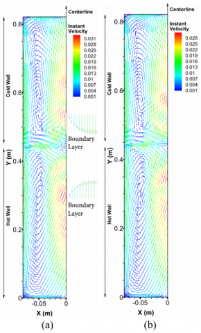
Figure 3 presents the instantaneous velocity vectors colored by their normalized magnitudes, the normalized temperature distributions and density contour in the reactor, showed in Figure 1a, by using the 2D k – ω SST turbulent model. The Boussinesq approximation and non-Boussinesq approach (temperature-dependent properties) were assumed for the working fluid in this section.
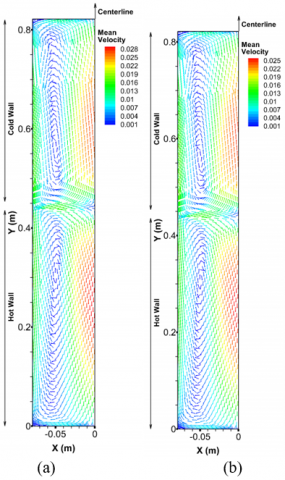
Figures 3a and 3b present the velocity vector map colored by the instantaneous velocity magnitude. The velocity vectors maps show flow patterns and flow direction through color magnitude. One needs to know that the author did not consider a same scale for the velocity magnitudes in the 2D and 3D results (Figures 3-7) as from the point of view of magnitudes, they were second in importance behind flow patterns and direction. A comparative inspection of Figures 3a and 3b shows that the results are indistinguishable in terms of having a similar flow pattern. For instance, flow with a high velocity magnitude moves in the central regions of the reactor. Yet, the flow with Boussinesq approximation implementation (Figure 3b), shows a relatively lower maximum velocity value compared to the simulation with temperature-dependent properties (Figure 3a). In order to better quantify the velocity distribution, the normalized time-averaged velocity magnitudes for these two cases (see Figures 4a and 4b) were calculated. The maximum normalized mean velocity magnitude over a time window of 100 s were 0.028 and 0.025 for the non-Boussinesq and Boussinesq cases, respectively. This shows that the maximum velocity using the Boussinesq approximation is lower than temperature-dependent properties due to the constant property assumption in this method. Although in using the Boussinesq approximation, the properties are assumed to be constant, but the results show an overall similarity between the two cases as the temperature gradient of 10 K does not change the working fluid’s properties significantly and there is a linear relation between the properties and temperature gradients. One can expect to see similar results for the numerical studies using the Boussinesq Approximation and temperature-dependent properties for the working fluid as long as the multiplication of thermal expansion coefficient in temperature gradient to be << 1.
Figure 3a also presents the boundary layer formation near the walls in two different locations in the reactor. These locations are illustrated in Figure 1a with B and C boxes. Each box with the dashed-line border represents the area between the wall and the flow in proximity of it. The flow moves upward in the lower hot wall due to the lower density while it moves downward in the upper cold zone as it is denser. These cold and hot streams meet each other near the insulator where the mixing happens (mixing zone).
The density gradient in the case with temperature-dependent properties, for the temperature gradient ($\Delta \mathrm{T}$ = 10 K), is about 4 kg/m3. This difference is mainly near the walls rather than the inner regions of the reactor. This implies that the buoyancy force is likely weak inside the regions far from the walls. In fact, the buoyancy force is dominant in the vicinity of the walls (boundary layer formation) while the shear force is the driven force in the central regions of the reactor. Note that the buoyancy force does exist in the regions far away the walls due to the little density gradient. As illustrated in Figure 3c, the flow with higher density values is located in the upper section of the reactor as the flow is cooler in that region. A similar conclusion is valid for the density distribution in the lower section of the reactor with regard to the reversed impact of higher temperature on the density distribution.
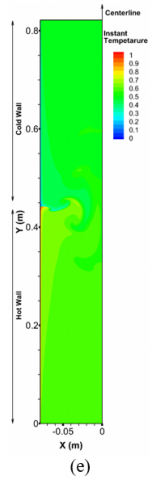
Figure 3. 2D instantaneous velocity, density and temperature distribution; $\Delta \mathrm{T}$= 10 K, with temperature-dependent properties at time = 1070 s (a, c and d), and with Boussiensq approximation at time = 1070 s (b and e)
Figures 3d and 3e depict the normalized instantaneous temperature contours of the cases with temperature- dependent properties and Boussinesq approximation, respectively. These two models provide a similar temperature distribution in the enclosure. The lower hot section of the reactor has a higher temperature while in the upper cold section of the reactor, flow with lower temperature exist. The current thermal map in the reactor confirms the density distribution in the reactor when the model with temperature-dependent properties was implemented in the numerical set up (Figure 3c).
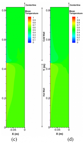
Figure 4. 2D time-averaged velocity and temperature distribution over a time-window of 100 s (970 - 1070 s); $\Delta \mathrm{T}$= 10 K, Non Boussinesq approximation (a and c), Boussiensq approximation (b and d)
Figures 4c and 4d present the time-averaged normalized temperature over a time window of 100 s for the both cases. As shown, they are very similar in terms of temperature distributions and this similarity indicates that both models (Boussinesq and non-Boussinesq) result in a similar thermal map inside the reactor.
Figure 5. 3D LES model using temperature-dependent properties, X-Y plane (Z = 0), DT = 10 K; (a) Velocity vector sized uniformly and colored by instantaneous velocity magnitude at time = 742 s (b) Normalized instantaneous temperature contour at time = 742 s (c) Normalized mean temperature contour over a time window of 100 s
4.2 Comparison of 3D Boussinesq and Non-Boussinesq LES simulations
The numerical results of 3D LES simulations, for the same boundary conditions and geometry size of Figure 1a, by considering temperature-dependent properties and the Boussinesq approximation for the working fluid inside the reactor (see Figure 1b) on the X-Y (Z = 0) plane are provided herein. Note that the author used the 3D k- ω SST RANS model for similar Ra and thermal boundary conditions in [13]. One can compare the distinct results of using 3D LES model instead of the 3D k-ω SST RANS model by comparing the thermal map inside the reactor.
Figures 5 and 6 depicts the velocity vector maps colored by their instantaneous normalized magnitudes, instantaneous and mean normalized temperature distributions on the X-Y plane for the non-Boussinesq and Boussinesq simulations, respectively. For the case with temperature-dependent properties, as shown in Figure 5a, there are multiple small vortices inside the domain which show that the flow is turbulent and has random movements. Unlike the 2D simulation, flow with higher velocity magnitude moves closer to the lateral walls rather than the central region of the reactor.
Figure 5b presents the normalized instantaneous temperature contour on the X-Y plane using the LES model in the numerical simulation considering temperature-dependent properties for the working fluid. It can be identified that the warmer fluid layers exist in the vicinity of the lower wall and overall, the temperature in the central regions of the reactor is uniform. The relatively uniform temperature distribution in the 3D result happens as the boundary layer is thin near the walls for the current Ra number and reactor size (in an under published study, the temperature distribution with the current boundary conditions and geometry size except the reactor diameter of 25.4 mm, the thermal map is totally different inside the reactor). In other words, the thermal resistance between the boundary layer zone and the bulk flow is not strong. The buoyancy force is the dominant force in the boundary layer regions and acts as the main driver of the flow in the reactor. However, the shear force is in charge of the flow movement in the central regions of the reactor. In fact, a large temperature gradient does not exist in the core regions of the reactor which results in a weak buoyant flow in those regions. The flow is relatively warmer in the upper section of the reactor compared to the lower one. This phenomenon shows a temperature inversion which means the cooler flow exists in the lower section of the reactor with warmer walls. The author extensively discussed about this physical phenomenon in ref. [13].
Figure 5c presents the normalized mean temperature over a time window of 100 s (642 s - 742 s) on X-Y plane using LES (Dynamic Smagorinsky) model with temperature-dependent properties for the working fluid in the simulation. A similar discussion of Figure 5b is again valid. The temperature inversion can be seen inside the reactor while the temperature is relatively uniform in each random radial section of the reactor.
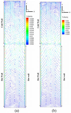
Figure 6 shows the velocity vector map colored by the instantaneous velocity magnitude, instantaneous and mean normalized temperature contours on X-Y plane while the Boussinesq approximation was considered in the numerical calculations for the working fluid.
Similar to Figure 5a, multiple small vortices exist inside the domain as a sign of turbulent flow. The cool and warm fluid flows meet in the mixing zone where they interact and exchange momentum and energy. The higher velocity magnitudes can be noticed near the lateral walls but not in the central region of the reactor (Figure 6a). Note that maximum velocity magnitude, similar to the 2D results, is lower (30%) for the case considering Boussinesq formulation rather the temperature-dependent properties for the working fluid.
Figure 6. 3D LES model using the Boussinesq approximation, X-Y plane (Z = 0) at time = 742 s, $\Delta \mathrm{T}$= 10 K; (a) Velocity vector sized uniformly and colored by instantaneous velocity magnitude (b) Normalized instantaneous temperature contour (c) Normalized time-averaged temperature contour over a time window of 100 s
Figure 6b shows the instantaneous normalized temperature on X-Y plane by considering the Boussinesq approximation for the working fluid. A similar discussion of Fig. 5b for the temperature distribution inside the reactor is valid. While the temperature distribution is uniform far away the walls, a temperature gradient exists near the lateral walls and it makes the buoyancy force as the dominant force near the lateral heated walls. A temperature inversion can be seen similar to the previous 3D simulation (Figure 5b).
Figure 6c shows the time-averaged normalized temperature on X-Y plane by considering the Boussinesq approximation for the working fluid. It clearly shows that during the time window of 100 s, a warmer fluid flow exists in the upper section of the reactor (temperature inversion).
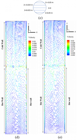
Figure 7 present the velocity vector maps colored by the instantaneous velocity magnitude for two more distinct times (680 s and 695 s) and on several planes (Z = 0 and Z ≠ 0). Figures 7a and 7b show that flow had different patterns on X-Y plane in different times. As fluid flow was turbulent, one can expect that different vortices (small or big) were formed in time and space and dissipated in another time (compare Figures 6a, 7a, 7b). In addition, maximum velocity magnitude on X-Y plane was changing due to the nature of flow in time (Figures 7a and 7b).
Figures 7d-7g presents the velocity vector maps colored by instantaneous velocity magnitude at t=695 s on four different planes parallel to X-Y plane (Z = 0.025 m, Z = - 0.025 m, Z = 0.05 m, Z = - 0.05 m; see Fig. 7c for their positions). It can be understood that flow patterns are different on those planes as flow is turbulent and random movements result in different velocity vectors and vortices on the planes.
Figure 7. Velocity vector sized uniformly and colored by instantaneous velocity magnitude using 3D LES model with the Boussinesq approximation, $\Delta \mathrm{T}$= 10 K; (a) X-Y plane (Z = 0) at time = 680 s (b) X-Y plane (Z = 0) at time = 695 s (c) Selected planes and their locations from the top view (d) plane Z = 0.025 m at time = 695 s (e) plane Z = -0.025 m at time = 695 s (f) plane Z = 0.05 m at time = 695 s (g) plane Z = -0.05 m at time = 695 s
Figure 8. 3D LES model with the Boussinesq approximation, X-Y plane (Z = 0), $\Delta \mathrm{T}$= 10 K; (a) Close view of instantaneous normalized temperature contour near the lower hot wall, (b) Zoomed-in view of the hot wall (box C in Figure 1a), (c) Close view of instantaneous normalized temperature contour in the vicinity of the mixing zone, (d) Close view of instantaneous normalized temperature contour near the upper cold wall, (e) Zoomed-in view of the cold wall (box B in Figure 1a)
It can be concluded that the thermal map inside the reactor is relatively similar for both cases (Boussinesq and Non-Boussinesq approach). The author considered five radial lines on X-Y (Z=0) plane to better show this similarity about the temperature distribution (along with the provided temperature contours). The location of each line is provided in Table 7.
Table 7. Location of different lines on X-Y plane
|
|
X (m) |
Y (m) |
Z (m) |
|
Line 1 |
[-0.079375, 0.079375] |
0.2 |
0 |
|
Line 2 |
[-0.079375, 0.079375] |
0.3 |
0 |
|
Line 3 |
[-0.079375, 0.079375] |
0.4 |
0 |
|
Line 4 |
[-0.079375, 0.079375] |
0.6 |
0 |
|
Line 5 |
[-0.079375, 0.079375] |
0.7 |
0 |
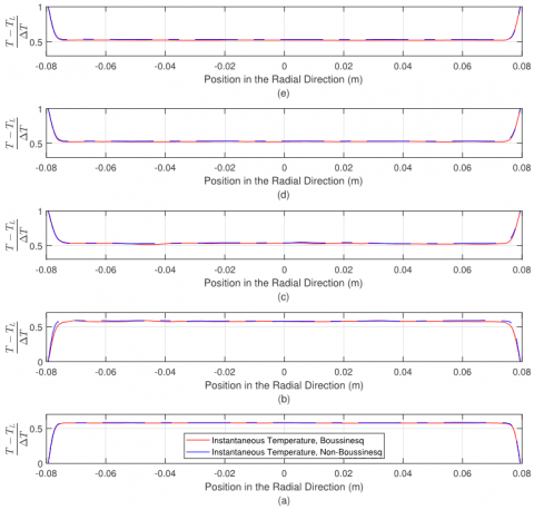
Figure 9. Instantaneous normalized temperature on different lines at time = 742 s; (a) Line 5 (b) Line 4 (c) Line 3 (d) Line 2 (e) Line 1
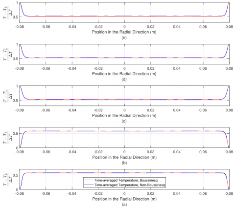
Figure 10. Time-averaged normalized temperature on different lines over a time window of 100 s; (a) Line 5 (b) Line 4 (c) Line 3 (d) Line 2 (e) Line 1
Figure 8 presents the general form of instantaneous normalized temperature contours near the lateral walls (hot zone, mixing zone, and cold zone). The flow is warmer in the vicinity of the lower hot zone, while near the upper cold zone flow holds the cooler fluid due to the applied thermal boundary condition. In the mixing zone, warmer and cooler flows meet each-other and exchange momentum and enthalpy. Note that far away the lateral walls, flow holds a relatively uniform temperature distribution inside the reactor (light green color).
Figures 9 and 10 show the instantaneous and time-averaged normalized temperature distribution across these five lines, respectively. As can be seen in these two figures, temperature is quite uniform in the interior regions of the reactor. However, there is a sharp temperature gradient near the walls (thermal boundary layer). These sharp temperature gradients correspond to the provide temperature contours in Figures 8a-8e. The sharp temperature gradient is the thermal boundary layer where flow temperature varies dramatically from the flow stream one to the wall temperature.
2D and 3D numerical simulations of natural convection in a laterally heated cylindrical enclosure were conducted using k- ω SST RANS and LES (Dynamic Smagorinsky) models by considering the Boussinesq approximation and non-Boussinesq (temperature-dependent properties) approach. The investigation used the CFD commercial software ANSYS FLUENT when a temperature gradient of 10 K was applied to a cylindrical geometry with the aspect ratio (L/D) of 5.17. The Prandtl number was Pr = 4.16 and the Rayleigh number was Ra = 2E7; note that the characteristic length for the Ra number was based on the ratio of the reactor’s volume to its lateral area as the characteristic length (Radius of the reactor/2). The numerical simulations were conducted using water as the working fluid. While Ammonia was the working fluid used in an ammonothermal crystal growth reactor, if one respects geometric (scaled dimensions in all directions by the same ratio) and dynamic similitude rules (a similar Ra number), then conclusions regarding flow and temperature patterns obtained from a numerical simulation done with water will apply to the GaN environment when geometric and dynamic similitude is respected.
Two main goals were considered in this study: The potential benefits of using the Boussinesq approximation instead of the temperature dependent properties for the working fluid and the potential benefits of using a 2D axisymmetric model instead of a full 3D domain.
Regarding the first goal, the fluid flow and thermal maps present comparisons of the results using the Boussinesq approximation and non-Boussinesq approach. It was shown while the velocity vector map and temperature distribution inside the enclosure exhibited similar patterns for both the 2D and 3D simulations, the Boussinesq approximation exhibited a relatively lower maximum velocity magnitude when compared with the non-Boussinesq results (up to 30%). It is important to note that based on the current study, the temperature gradient between the hot and cold sides should be equal or less than 10 K for both methods to yield similar results. As a future work, one can increase the applied temperature gradient on the lateral walls (for instance 20 K, 30 K, 40 K) and compare the results using both methods (Boussinesq approximation ad temperature-dependent properties.
For the second goal, the 3D simulation was implemented to investigate the effect(s) of using a 3D model instead of a 2D axisymmetric one. In fact, the results of this particular effort yielded one of the more important findings of this study. The comparison between the 2D k-ω SST RANS and 3D LES (Dynamic Smagorinsky) models, both using Boussinesq and Non-Boussinesq approach, showed that the velocity vector and temperature maps were significantly different in the 2D from the 3D numerical results. In the 3D model, unlike the results of the 2D model, smaller vortices and different fluid flow patterns were noticed, while the maximum velocity values shifted from the central regions of the reactor, towards the walls of the enclosure. It was also found that 3D flow was not axisymmetric despite the axisymmetric boundary conditions (see Figures 4a, 4b, 5a, and 6a). This can be attributed to the turbulence and the three-dimensionality of the flow; the latter obviously was missing in the 2D axisymmetric results.
The 3D temperature distribution was notably different from the 2D model result. The difference between these two thermal distributions (2D and 3D models) lies on the physics of the problem at this Ra number, reactor size, and the outcomes of the full 3D simulation which considers the effects of the circumferential gradients in velocity and temperature distributions. In the 3D model, warmer flows circulated closer to the walls unlike in the 2D model’s outcome (buoyancy force versus shear force). In the 3D results the buoyancy force was only dominant near the lateral walls while the core regions were driven by shear force (buoyancy force was weak in the central regions).
The authors believe that a 3D model for simulations is the only way to get a proper rendition of the velocity vector and temperature maps in the study of turbulent Boussinesq or non-Boussinesq flows, as a 2D axisymmetric model for a laterally heated cylindrical ammonothermal crystal growth reactor does not give results consistent with a 3D model (in the diametral longitudinal cross section) run under the same boundary conditions, temperature differential, turbulence model and Ra number. It is possible that for the laminar regime the 3D and 2D axisymmetric results are more coincident, but turbulence definitely rules out this possibility. In authors’ view, the 2D simulations may be offering guidance, but they are off as far as accuracy is concerned.
It is worth noting certain scale and flow formations reform somewhat periodically (quasi-steady flow), even though not exactly the same, but a true steady state never sets in for the presented geometry, Ra magnitude and provided boundary conditions.
This paper is based upon work supported by the National Science Foundation under Grant No. 1336700.
|
D |
Diameter of the reactor, m |
|
CP |
Specific heat, J. kg-1. K-1 |
|
g |
Gravitational acceleration, m. s-2 |
|
k |
Thermal conductivity, W.m-1. K-1 |
|
E |
Energy, kg.m2. s-2 |
|
H |
Enthalpy, kg.m2. s-2 |
|
k |
Turbulent kinetic energy, m2. s-2 |
|
Keff |
Total thermal conductivity, W.m-1. K-1 |
|
L |
Characteristic length, m |
|
Nu |
Nusselt number |
|
Gr |
Grashof number |
|
Pr |
Prandtl number |
|
Ra |
Rayleigh number |
|
t |
Time, s |
|
T |
Temperature, K |
|
Ρ |
Density, kg.m-3 |
|
Τ |
Shear stress, N.m-2 |
|
Pk |
Generation of turbulence kinetic energy, m2. s-2 |
|
Greek symbols |
|
|
$\alpha$ |
Thermal diffusivity, m2. s-1 |
|
$\alpha_{T}$ |
Turbulent thermal diffusivity, m2. s-1 |
|
$\beta$ |
Thermal expansion coefficient, K-1 |
|
Ɵ |
Dimensionless temperature |
|
µ |
Dynamic viscosity, kg. m-1. s-1 |
|
µt |
Eddy viscosity, m2.s-1 |
|
ν |
Kinematic viscosity, m2. s-1 |
|
Ф |
Scalar quantity |
|
γ |
Porosity |
|
$\omega$ |
Specific dissipation rate, s-1 |
|
$\varepsilon$ |
Dissipation of turbulent kinetic energy, m2.s-3 |
[1] Ehrentraut, D., Meissner, E., Bockowski, M. (Ed). (2010). Technology of Gallium Nitride Crystal Growth. Springer Science & Business Media.
[2] Bodoia, J.R., Osterle, J.F. (1962). The development of free convection between heated vertical plates. Journal of Heat Transfer, 84(1): 40-43. https://doi.org/10.1115/1.3684288
[3] Ostrach, S. (1988). Natural convection in enclosures. Journal of Heat Transfer, 110(4b): 1175-1190. https://doi.org/10.1115/1.3250619
[4] Fusegi, T., Hyun, J.M., Kuwahara, K. (1991). A numerical study of 3D natural convection in a cube: effects of the horizontal thermal boundary conditions. Fluid Dynamics Research, 8(5-6): 221. https://doi.org/10.1016/0169-5983(91)90044-J
[5] Salmun, H. (1995). Convection patterns in a triangular domain. International Journal of Heat and Mass Transfer, 38(2): 351-362. https://doi.org/10.1016/0017-9310(95)90029-2
[6] Li, H.M., Braun, M.J., Evans, E.A., Wang, G.X., Paudel, G., Miller, J. (2005). Natural convection flow structures and heat transfer in a model hydrothermal growth reactor. International Journal of Heat and Fluid Flow, 26(1): 45-55. https://doi.org/10.1016/j.ijheatfluidflow.2004.06.005
[7] Badr, H.M., Habib, M.A., Anwar, S., Ben-Mansour, R., Said, S.A.M. (2006). Turbulent natural convection in vertical parallel-plate channels. Heat and Mass Transfer, 43(1): 73-84. https://doi.org/10.1007/s00231-006-0084-z
[8] Li, H.M., Braun, M.J., Xing, C.H. (2006). Fluid flow and heat transfer in a cylindrical model hydrothermal reactor. Journal of Crystal Growth, 289(1): 207-216. https://doi.org/10.1016/j.jcrysgro.2005.10.113
[9] Daverat, C., Pabiou, H., Menezo, C., Bouia, H., Xin, S. (2013). Experimental investigation of turbulent natural convection in a vertical water channel with symmetric heating: Flow and heat transfer. Experimental Thermal and Fluid Science, 44: 182-193. https://doi.org/10.1016/j.expthermflusci.2012.05.018
[10] Enayati, H., Chandy, A.J., Braun, M.J. (2015). Numerical simulations of natural convection in a laterally-heated cylindrical reactor. American Society of Thermal and Fluids Engineers, NYC. https://doi.org/10.1615/TFESC1.cmd.012704
[11] Enayati, H., Chandy, A.J., Braun, M.J. (2016). Numerical simulations of transitional and turbulent natural convection in laterally heated cylindrical enclosures for crystal growth. Numerical Heat Transfer, Part A: Applications, 70(11): 1195-1212. https://doi.org/10.1080/10407782.2016.1230378
[12] Enayati, H., Chandy, A.J., Braun, M.J. (2016). Numerical simulations of turbulent natural convection in laterally-heated cylindrical enclosures with baffles for crystal growth. In ASME 2016 International Mechanical Engineering Congress and Exposition, pages V008T10A052–V008T10A052. American Society of Mechanical Engineers. https://doi.org/10.1115/IMECE2016-66106
[13] Enayati, H., Chandy, A.J., Braun, M.J., Horning, N. (2017). 3D large eddy simulation (les) calculations and experiments of natural convection in a laterally-heated cylindrical enclosure for crystal growth. International Journal of Thermal Sciences, 116: 1-21. https://doi.org/10.1016/j.ijthermalsci.2017.01.025
[14] Enayati, H., Chandy, A.J., Braun, M.J. (2018). Large eddy simulation (les) calculations of natural convection in cylindrical enclosures with rack and seeds for crystal growth applications. International Journal of Thermal Sciences, 123: 42-57. https://doi.org/10.1016/j.ijthermalsci.2017.08.025
[15] Enayati, H., Braun, M.J., Chandy, A.J. (2017). Numerical simulations of porous medium with different permeabilities and positions in a laterally-heated cylindrical enclosure for crystal growth. Journal of Crystal Growth, 483: 65-80. https://doi.org/10.1016/j.jcrysgro.2017.11.019
[16] Enayati, H., Chandy, A.J., Braun, M.J. (2017). Three-dimensional large eddy simulations of natural convection in laterally heated cylindrical enclosures with racks and seeds for crystal growth. Second Thermal and Fluids Engineering Conference, pp. 719-732. https://doi.org/10.1615/TFEC2017.cfd.017674
[17] Enayati, H. (2019). Numerical flow and thermal simulations of natural convection flow in laterally- heated cylindrical enclosures for crystal growth. PhD thesis, University of Akron.
[18] Enayati, H. (2020). Effect of reactor size in a laterally-heated cylindrical reactor. International Journal of Heat and Technology, 38(2): 275-284. https://doi.org/10.18280/ijht.380201
[19] Suslov, S.A., Paolucci, S. (1995). Stability of natural convection flow in a tall vertical enclosure under non-boussinesq conditions. International Journal of Heat and Mass Transfer, 38(12): 2143-2157. https://doi.org/10.1016/0017-9310(94)00348-Y
[20] Vierendeels, J., Merci, B., Dick, E. (2004). A multigrid method for natural convective heat transfer with large temperature differences. Journal of Computational and Applied Mathematics, 168(1): 509-517. https://doi.org/10.1016/j.cam.2003.08.081
[21] Othman, S. (2005). A numerical study of transient natural convection of water near its density extremum. PhD thesis, University of Strathclyde.
[22] Szewc, K., Pozorski, J., Minier, J.P. (2012). Analysis of the incompressibility constraint in the smoothed particle hydrodynamics method. International Journal for Numerical Methods in Engineering, 92(4): 343-369. https://doi.org/10.1002/nme.4339
[23] Tong, W., Koster, J.N. (1993). Natural convection of water in a rectangular cavity including density inversion. International Journal of Heat and Fluid Flow, 14(4): 366-375. https://doi.org/10.1016/0142-727X(93)90010-K
[24] Saber, H., Messaoud, G., Madiha, B. (2014). Numerical study of natural convection in a square cavity under non-boussinesq conditions. Thermal Science, 20(5): 84-84. https://doi.org/10.2298/TSCI130810084H
[25] Paulucci, S. (1982). On the filtering of sound from the navier-stokes equations, sandia national labs. In Tech. Rep. Report SAND-82-8257. https://ui.adsabs.harvard.edu/abs/1982STIN...8326036P/abstract.
[26] Chenoweth, D.R., Paolucci, S. (1986). Natural convection in an enclosed vertical air layer with large horizontal temperature differences. Journal of Fluid Mechanics, 169: 173-210. https://doi.org/10.1017/S0022112086000587
[27] Sharma, N., Diaz, G. (2015). Heat transfer and flow-pattern formation in a cylindrical cell with partially immersed heating element. American Journal of Heat and Mass Transfer, 2(1): 31-41. https://doi.org/10.7726/AJHMT.2015.1003
[28] Kizildag, D., Rodr´ıguez, I., Oliva, A., Lehmkuhl, O. (2014). Limits of the oberbeck–boussinesq approximation in a tall differentially heated cavity filled with water. International Journal of Heat and Mass Transfer, 68: 489-499. https://doi.org/10.1016/j.ijheatmasstransfer.2013.09.046
[29] White, F.M. (2003). Fluid Mechanics. 5th. Boston: McGraw-Hill Book Company.
[30] Pramuditya, S. Water thermodynamic properties. https://syeilendrapramuditya.wordpress.com/2011/08/20/water- thermodynamic-properties/, accessed on Oct. 2, 2021.